Beyond Constant Error: Heteroscedastic Bayesian Model Combination for Modeling Unmeasured Nuclei

Source: arXiv:2607.14039 · Published 2026-07-15 · By B. Knight, S. Lalit, P. Giuliani, K. Godbey, W. Nazarewicz, A. Ravlić et al.

TL;DR

The heteroscedastic BMC leverages principal component analysis (PCA) of the model ensemble outputs to identify features that correlate with prediction error, such as distance in PC space from the training data and the variance between individual models’ predictions. By modeling uncertainty as a function of these features, the framework accounts for degradation of predictive power with extrapolation. The authors validate this approach on synthetic benchmarks where one model is held out as ground truth, demonstrating improved calibration (lower mean absolute calibration error) and better statistical metrics like reduced chi-square values closer to unity. Application to experimental nuclear data from the AME2020 compilation confirms that heteroscedastic BMC reduces root mean squared error versus single models and provides superior calibrated uncertainty intervals in the extrapolation domain near nuclei with Z=46–52. This work represents a significant advance in principled, statistically robust uncertainty quantification for nuclear physics predictions in difficult extrapolation regimes.

Key findings

• Heteroscedastic Bayesian Model Combination (HeEM) yields superior calibration metrics compared to homoscedastic error model (HoEM), with reduced chi-square scores closer to unity across validation sets (see Table IV).
• Using features: distance in principal component (PC) space and model variance as predictors of error scale allows dynamic uncertainty quantification that adapts to location in nuclear chart.
• Synthetic data tests, in which one nuclear model serves as ground truth, show that HeEM reduces mean absolute calibration error (MACE) on average from 10.9 (HoEM) to 7.3 (HeEM Linear) in the near-extrapolation validation set (Table II).
• BMC combining six nuclear energy density functional models outperforms all individual models on root mean squared error (RMSE) across neutron and proton separation energies in the experimental holdout set (RMSE ~0.22–0.37 MeV vs individual models typically 0.35–0.80 MeV, Table III).
• The linear form of the heteroscedastic error model achieves comparable or better performance than a quadratic variant, while being more parsimonious.
• The heteroscedastic model naturally captures larger uncertainties for challenging odd-N nuclei where models diverge, unlike the constant uncertainty band of HoEM (Fig. 7).
• Validation-set metrics (RMSE, MACE, reduced chi-square) are predictive of prediction-set (extrapolation) performance, supporting the robustness of the heteroscedastic approach.

Threat model

n/a — The paper does not address an adversarial threat model. The focus is on epistemic uncertainty quantification of theoretical nuclear models to improve predictive accuracy and calibrated confidence intervals when extrapolating to experimentally inaccessible nuclei.

Methodology — deep read

The authors consider the problem of predicting nuclear binding energy related observables (one- and two-neutron/proton separation energies and alpha decay Q-values) for nuclei with proton number Z=46-52, including nuclei without experimental data (extrapolation domain).

The threat model is inherent uncertainty due to incomplete physics and limited calibration data; they assume no adversarial interaction but focus on robust model combination and uncertainty quantification in deep extrapolation.

Data comes from six nuclear energy density functionals (EDFs) with varying physics assumptions and calibration protocols: three covariant EDFs (DD-PC1, DD-PCX, DD-ME2), two Skyrme EDFs (UNEDF1, UNEDF2), and one Fayans EDF (Fy(IVP)). The dataset of observables includes experimentally measured (AME2020) nuclei near the valley of stability and extensive predictions for unmeasured nuclei.

Datasets are partitioned into training (core well-measured isotopes), validation (boundary isotopes near training limits), and prediction (extrapolation) sets.

The Bayesian Model Combination (BMC) framework first centers each model's predictions by subtracting the mean prediction vector. Then, singular value decomposition (SVD) extracts principal components (PCs) representing dominant variability axes in model predictions. The BMC combines the average model prediction with a linear combination of these retained PCs weighted by parameters 'b' estimated in a Bayesian fashion using the training data.

Errors are modeled as Gaussian noise with zero mean and a data-dependent scale parameter sigma_i. Unlike prior work assuming homoscedastic constant variance sigma0 for all data (HoEM), this paper models sigma_i heteroscedastically as a function g(z_i; Λ), where z_i is a vector of features per data point, and Λ are parameters learned from data.

Two key features for g are: (1) distance d_i of the nucleus in PC space from the nearest training data and (2) variance v_i of individual model predictions at that point, quantifying model disagreement. Different parametric forms of g are explored: constant (HoEM), linear, and quadratic functions of d_i and v_i.

Inference samples the posterior distribution over b and Λ using a Metropolis-within-Gibbs Markov Chain Monte Carlo (MCMC) sampler, enabling uncertainty propagation.

Evaluation metrics include RMSE for mean prediction accuracy, reduced chi-square for variance calibration, and mean absolute calibration error (MACE) assessing empirical coverage of predicted credible intervals.

Synthetic validation is conducted by treating each EDF model in turn as ground truth and fitting the BMC to the remaining models with synthetic data corresponding to the held-out model’s predictions. This measures ability of heteroscedastic BMC to generalize in extrapolation.

Application to the experimental AME2020 data focuses on Z=46–52 isotopes, comparing HoEM and heteroscedastic BMC variants on validation sets and deep extrapolations.

Results show that heteroscedastic BMC better balances uncertainty across training and extrapolation domains, avoiding overly conservative or overconfident intervals and better resolving heterogeneous uncertainty across nuclear chains. The linear heteroscedastic model is preferred as the best tradeoff between complexity and performance.

Code and detailed parameter settings are not explicitly stated as released, though methodological steps are clear. The approach is reproducible given access to the EDF predictions and experimental benchmarks.

Example end-to-end: For S1n neutron separation energies on tin isotopes, model predictions from six EDFs are combined via BMC with weights fit on training data. Heteroscedastic error scale in PC space dynamically grows uncertainty with distance and model disagreement, leading to calibrated credible intervals that encompass true synthetic or experimental values in the validation and extrapolation sets where individual EDFs diverge strongly.

Technical innovations

• Introduction of a heteroscedastic Bayesian Model Combination framework that models predictive uncertainty as a dynamic quantity varying with features rather than assuming constant error variance.
• Use of principal component analysis (PCA) on the ensemble model prediction deviations to define a continuous physical feature space for error scale modulation.
• Construction of interpretable uncertainty predictors from model disagreement variance and PC-space distance to training data, allowing uncertainty to increase naturally with extrapolation difficulty.
• Integration of a Metropolis-within-Gibbs Bayesian inference sampler to sample posterior distributions over both model combination weights and heteroscedastic error parameters jointly.

Datasets

• AME2020 — experimental atomic mass evaluation — public nuclear data compilation
• Synthetic datasets — generated by treating one EDF model as ground truth to validate extrapolation

Baselines vs proposed

• Individual EDF models: RMSE on neutron separation energies ranged from 0.35 to 0.80 MeV versus BMC (HoEM) RMSE ~0.22 MeV and BMC (Linear HeEM) RMSE ~0.22 MeV (Table III)
• HoEM: reduced chi-square on validation ~0.49–0.69 (proton/neutron Sep energies) versus Linear HeEM achieving closer to unity ~0.71–0.86 (Table IV)
• Synthetic test MACE validation: HoEM = ~5.88 to 10.90 versus HeEM Linear = ~4.15 to 7.31 (Table II)

Figures from the paper

Figures are reproduced from the source paper for academic discussion. Original copyright: the paper authors. See arXiv:2607.14039.

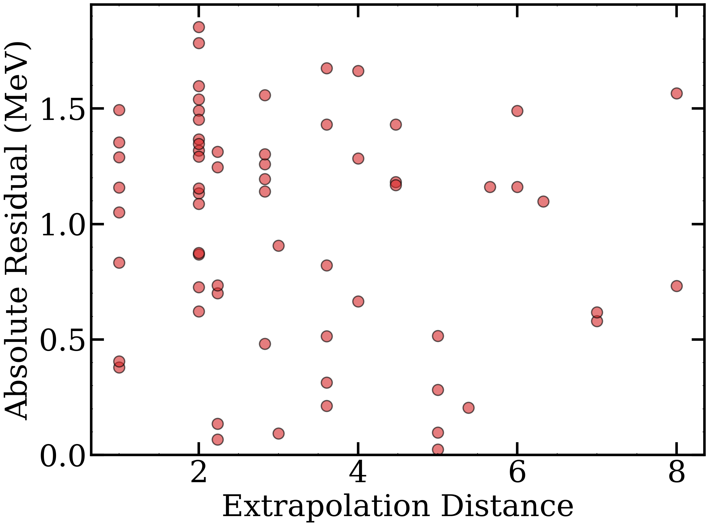
Fig 2: For each nucleus in the validation set, plotted is the

Limitations

• Validation primarily focuses on relatively narrow isotopic chains (Z=46–52), limiting immediate generalization to full nuclear chart extremes.
• Uncertainty calibration relies on synthetic data experiments where one model acts as ground truth—a proxy for real experimental error but no perfect truth model exists.
• The approach assumes Gaussian errors and conditional independence of residuals, which may not fully capture complex physical correlations or systematic model biases.
• No explicit adversarial or robustness testing against purposeful perturbation or model misspecification is performed.
• The quadratic heteroscedastic error model shows inconsistent improvements and sometimes worse calibration, demonstrating sensitivity to functional form choice.
• Code release and dataset availability are not clearly stated, potentially limiting reproducibility outside groups with access to nuclear model outputs.

Open questions / follow-ons

• How well does the heteroscedastic BMC framework generalize when applied to other nuclear regions, especially superheavy or far neutron-rich nuclei where models diverge more?
• Can more sophisticated nonlinear or nonparametric heteroscedastic models, e.g., Gaussian processes, further improve uncertainty calibration and provide physical insight?
• How robust are model combination weights and uncertainty estimates to inclusion or exclusion of particular nuclear models or model classes?
• Can this approach be extended to model correlated residuals among neighboring nuclei to exploit known nuclear structure systematics better?

Why it matters for bot defense

While primarily a domain-specific advancement in nuclear physics model uncertainty quantification, the technical innovation of heteroscedastic Bayesian model combination addresses a common problem in bot-defense ML: modeling uncertainty that varies with input features rather than assuming global homoscedastic noise. Bot-detection systems often face distributional shifts in usage patterns and adversarial attempts, analogous to nuclear model extrapolations beyond data support. Applying heteroscedastic model combination could help improve confidence calibration under shifts or rare events in bot detection ensembles by combining multiple imperfect detectors with input-dependent uncertainty scaling. Practitioners might consider integrating PC-based latent feature spaces and inter-model variance as predictors of model confidence degradation, enhancing robustness of ensemble predictions. The Bayesian inference machinery affords principled uncertainty quantification important in high-stakes bot defense decisions. However, adaptation would require mapping key features relevant to traffic shifts and adversarial input properties.

Cite

@article{arxiv2607_14039,
  title={ Beyond Constant Error: Heteroscedastic Bayesian Model Combination for Modeling Unmeasured Nuclei },
  author={ B. Knight and S. Lalit and P. Giuliani and K. Godbey and W. Nazarewicz and A. Ravlić and P. -G. Reinhard },
  journal={arXiv preprint arXiv:2607.14039},
  year={ 2026 },
  url={https://arxiv.org/abs/2607.14039}
}

Read the full paper

• arXiv:2607.14039 (abstract)
• arXiv:2607.14039 (PDF)