
Recovering Governing Equations from Solution Data: Identifiability Bounds for Linear and Nonlinear ODEs
Source: arXiv:2606.27285 · Published 2026-06-25 · By Yang Pan, Helmut Bölcskei
TL;DR
This paper addresses the foundational theoretical problem of when and how governing ordinary differential equations (ODEs) can be uniquely and stably recovered from observed solution trajectories. While significant algorithmic work exists on discovering equations from data, there is comparatively little rigor on identifiability conditions and sample complexity bounds for equation learning. The authors fill this gap by introducing the Hausdorff distance between sets of solution trajectories as a natural, minimax metric to measure closeness of ODEs themselves. They derive identifiability bounds connecting distances between structure equations (e.g., matrices for linear ODEs, Lipschitz vector fields for nonlinear ODEs) and their solution sets, rigorously proving both lower and upper bounds on the Hausdorff distance for several broad ODE classes. The analysis yields fundamental uniqueness (identification) and stability guarantees for a wide range of linear and nonlinear ODEs characterized by Lipschitz or Hölder continuity assumptions. They further derive sample complexity and metric entropy results quantifying how much solution data is needed to reliably learn the governing equation, providing theoretical foundations absent from prior scientific machine learning literature.
Key findings
- For first-order, d-dimensional linear ODEs with structure matrices A and ˜A, the Hausdorff distance hd between their solution sets satisfies c∥A−˜A∥₂ ≤ hd ≤ C∥A−˜A∥₂ for constants c, C depending only on system parameters (Theorem 4.1).
- A set of initial conditions that forms a basis (frame) for ℝ^d is necessary and sufficient for unique identification of linear ODE structure matrices from solution data.
- For Lipschitz nonlinear ODEs with vector fields f, ˜f over a compact initial condition set Q, the Hausdorff distance satisfies min(C₁∥f−˜f∥²_{L∞(Q)}, C₂∥f−˜f∥{L∞(Q)}) ≤ hd ≤ C₃∥f−˜f∥ (Theorem 4.2).
- Identifiability depends on access to solution trajectories over sufficiently rich initial condition sets; without spanning initial conditions, different ODEs may share identical solution sets (e.g., Lemma 4.4).
- Quantitative sample complexity estimates connect metric entropy of ODE classes under the Hausdorff metric to the number of solution trajectories needed to recover the governing equation reliably.
- The Hausdorff metric on solution sets naturally captures the minimax structure of the identification problem by quantifying worst-case solution trajectory deviations over initial conditions.
- Examples demonstrate that small changes in ODE parameters cause bounded perturbations in solution sets, and conversely small solution set distances guarantee structural closeness under assumptions, showing stability.
- Even nonlinear, Lipschitz-continuous vector fields enjoy stable identifiability via these bounds under sufficient initial condition coverage.
Threat model
An adversary is a learner observing solution trajectories generated by an unknown ODE from initial conditions within a known set. The adversary aims to recover the underlying vector field governing the ODE uniquely and stably. The adversary can query or access multiple solution observations over fixed time. It cannot observe solutions outside the initial condition set or with arbitrary perturbations, and assumes knowledge of the ODE class (linear, Lipschitz etc.).
Methodology — deep read
Threat model & assumptions: The adversary corresponds to a learning algorithm that attempts to recover the ground-truth ODE vector field f from observed solution trajectories. The setup assumes autonomous ODEs of order m with state dimension d: x^{(m)} = f(x^{(m-1)}, ..., x, t). The unknown structure function f lies within a known class F (e.g., linear, Lipschitz continuous). The adversary observes potentially multiple solution trajectories initialized at various initial conditions and seeks to determine f uniquely and stably. Importantly, no assumptions are made on fixed parameterizations of f to remain representation independent. Adversary capabilities include access to trajectory data over time horizon T from initial conditions in a set I ⊂ ℝ^{md}.
Data: The data considered are function solution sets B_I(O_f) consisting of all solution trajectories of ODE O_f starting from initial conditions in I over fixed time interval [0,T]. No explicit finite dataset is assumed at the theoretical level; the analysis quantifies how many sample trajectories (i.e., initial conditions and observation times) suffice for identification via metric entropy.
Architecture/algorithm: The paper does not propose a specific learning algorithm. Instead, it defines a metric space for ODEs using the Hausdorff distance hd_I between their solution sets under a ∥·∥_{C^{m-1}} norm. This metric measures worst-case distances between trajectories generated by two ODEs across all initial conditions in I. The central insight is to relate hd_I to distances between structure functions ∥f_1 - f_2∥. For linear ODEs, this corresponds to the matrix norm difference between A and ˜A. For nonlinear ODEs, this is the L∞ difference of vector fields over Q.
Training regime: The theoretical analysis is non-algorithmic and does not involve training. Instead, it derives upper and lower bounds on hd_I in terms of structure distances, uses Gronwall-type inequalities and matrix exponentials bounds for linear systems, and employs compactness and Lipschitz continuity arguments for nonlinear cases.
Evaluation protocol: The effectiveness of identifiability is quantified by explicit inequalities bounding the Hausdorff distance hd_I of solution sets between two ODEs in terms of the structural distance between their vector fields. The paper establishes matching lower and upper bounds (Theorems 4.1, 4.2) proving stability and uniqueness. These bounds also imply sample complexity by metric entropy calculations related to how many initial conditions are needed for a target accuracy.
Reproducibility: The paper is theoretical and does not release code or datasets. Results depend on known mathematical inequalities and properties of linear algebra and functional analysis. Example proofs are provided for lemmas about matrix exponentials, frames of initial conditions, and Gronwall bounds. Concrete examples include linear second-order oscillators and Lipschitz functions illustrating ill-posedness without sufficient initial coverage.
Concrete example (end-to-end): For first-order linear ODEs x' = A x and x' = ˜A x with A, ˜A ∈ ℝ^{d×d}, the authors use matrix exponentials to bound the max difference between solution trajectories over t ∈ [0,T] and compact initial conditions ∥x_0∥ ≤ D. Applying the inequality ∥e^{A t} - e^{˜A t}∥ ≤ t e^{K t} ∥A - ˜A∥ (Lemma B.7), they derive upper bounds on the Hausdorff distance of solution sets. Through quadratic form arguments and eigenvalue bounds (Lemma B.8), they produce matching lower bounds, establishing identifiability bounds linking operator norm differences of A, ˜A and trajectory differences. This example illustrates the method of relating solution closeness to structure closeness quantitatively for linear systems.
Technical innovations
- Introduction of the Hausdorff distance on solution sets of ODEs as a natural metric capturing worst-case deviations over initial conditions for identifiability analysis.
- Derivation of matching lower and upper bounds relating the Hausdorff distance between solution sets and the norm difference between structure equations for linear and nonlinear ODE classes.
- Identification of completeness (spanning frame) of initial condition sets as both necessary and sufficient for unique identification of linear ODE structure matrices.
- Metric entropy and sample complexity bounds for classes of ODEs under the Hausdorff metric, quantifying how many solution observations are necessary for stable recovery.
Baselines vs proposed
- No empirical baselines; comparisons are theoretical and involve bounding Hausdorff distance vs structural norm differences for ODE classes.
Figures from the paper
Figures are reproduced from the source paper for academic discussion. Original copyright: the paper authors. See arXiv:2606.27285.
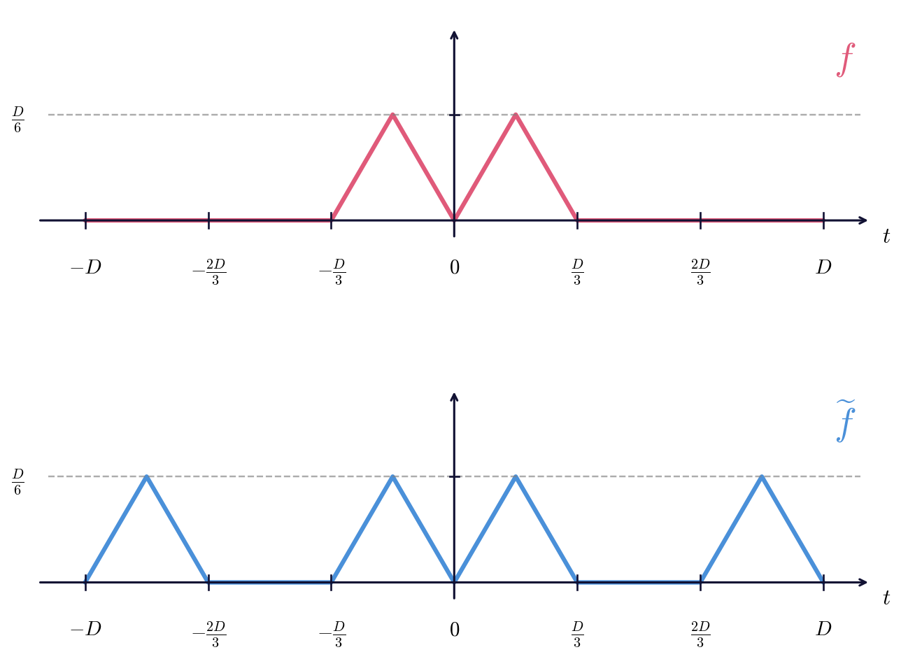
Fig 1: Lipschitz functions f and ˜f
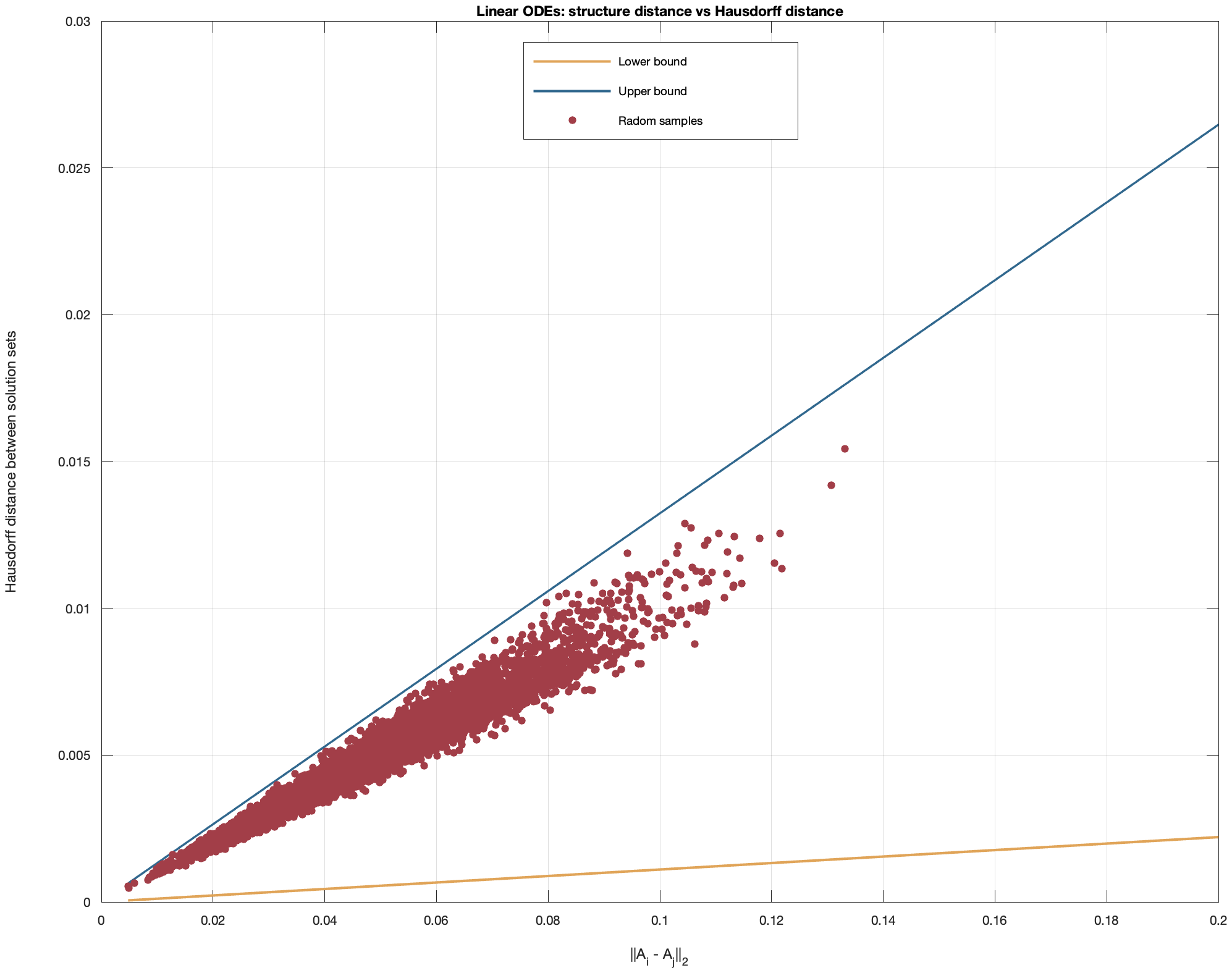
Fig 2: Red points represent the randomly generated samples. Yellow and blue
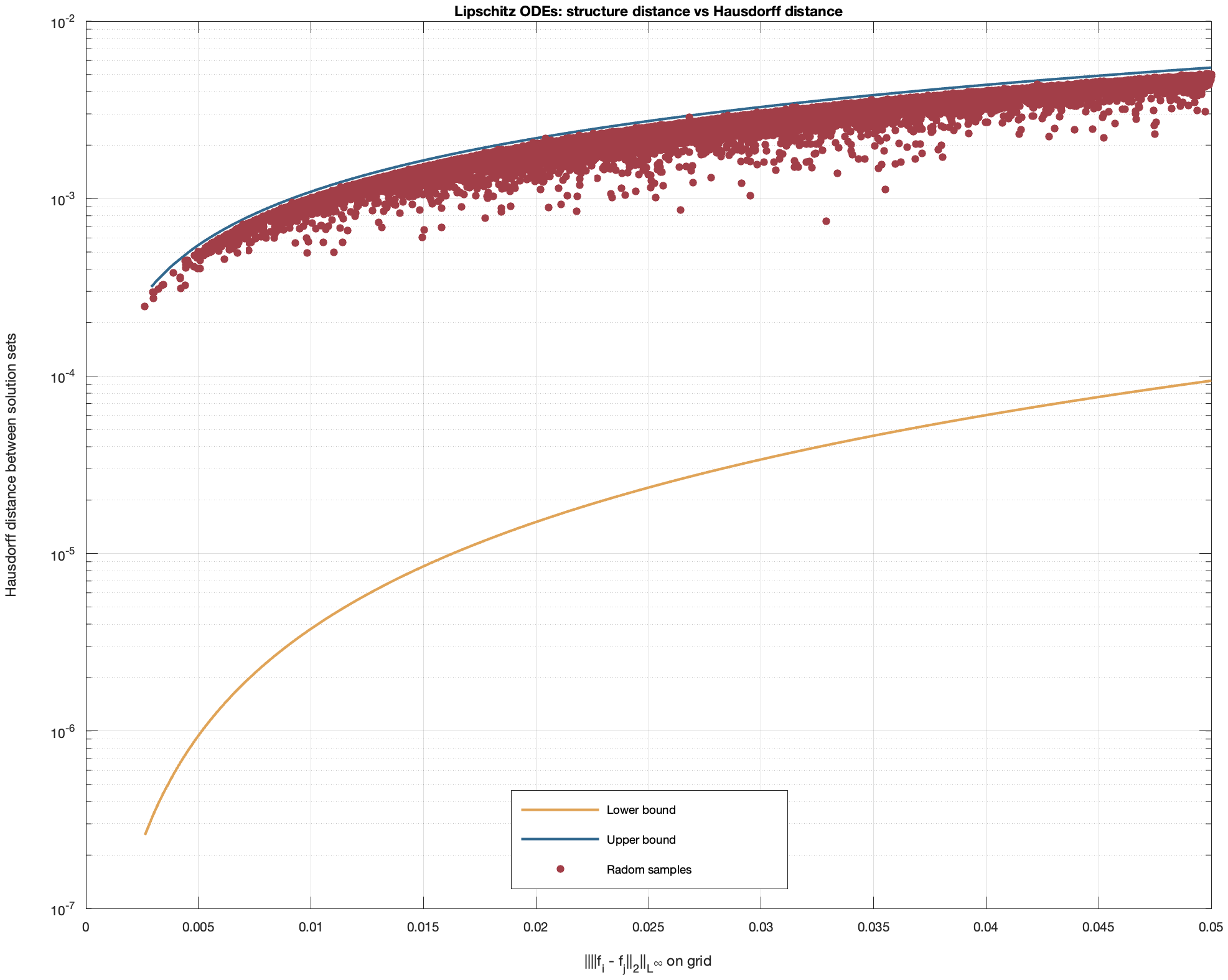
Fig 3: reports, for all indices i, j P t1, . . . , 600u, the pairwise Hausdorff dis-
Limitations
- Analysis limited to autonomous ODEs; extension to PDEs and non-autonomous systems is left for future work.
- Results assume access to rich sets of initial conditions spanning state space; limited initial condition coverage leads to identifiability issues.
- No explicit evaluation on noisy or finite, discretely sampled data; analysis is in the idealized continuous trajectory setting.
- Nonlinear results hold under Lipschitz and Hölder continuity assumptions; more general function classes are not addressed.
- No proposed practical algorithms or numerical schemes; the work focuses on theoretical identifiability rather than learning procedure design.
Open questions / follow-ons
- How to extend identifiability and complexity bounds from ODEs to partial differential equations (PDEs) with infinite-dimensional states?
- How do noise, finite sampling, and measurement error affect identifiability and sample complexity quantitatively?
- Can these theoretical metrics and bounds guide the design of practical identification algorithms that provably achieve stable recovery?
- How do non-autonomous ODEs, time-varying parameters, or stochastic dynamics impact identifiability frameworks based on solution set metrics?
Why it matters for bot defense
This paper provides rigorous theoretical underpinnings for the fundamental problem of uniquely recovering dynamical system models from observed trajectories, which is conceptually related to distinguishing legitimate (human or legitimate bot) behavior from adversarial or spoofed patterns. Bot defense systems increasingly rely on dynamic behavioral modeling, and understanding when observed data can uniquely identify underlying 'governing equations' is crucial for discriminative robustness. The introduction of Hausdorff distance over solution trajectories as a minimax metric formalizes how different differential equation models can be reliably distinguished in practice.
Practitioners designing CAPTCHAs or bot-detection engines that depend on modeling user interaction dynamics can benefit from these identifiability bounds, as they highlight the importance of sampling sufficiently rich initial states (e.g., varied session contexts or environmental conditions) and measuring trajectory similarity in a manner capturing worst-case deviations. The sample complexity analysis implies how much observational diversity is necessary for stable, unique detection capabilities. Though the work does not present direct algorithmic methods, its theoretical insights critically inform when learned dynamic models underlying behavior-based CAPTCHA solutions can be expected to generalize uniquely rather than overfit ambiguous data.
Cite
@article{arxiv2606_27285,
  title={ Recovering Governing Equations from Solution Data: Identifiability Bounds for Linear and Nonlinear ODEs },
  author={ Yang Pan and Helmut Bölcskei },
  journal={arXiv preprint arXiv:2606.27285},
  year={ 2026 },
  url={https://arxiv.org/abs/2606.27285}
}