Zero-Shot Imagined Speech Decoding via Imagined-to-Listened MEG Mapping

Source: arXiv:2605.08075 · Published 2026-05-08 · By Maryam Maghsoudi, Shihab Shamma

TL;DR

This paper tackles one of the hardest problems in non-invasive brain-computer interfaces: decoding imagined speech from MEG without requiring labeled imagined-speech training data. The core difficulty is that imagined neural signals are temporally imprecise, low SNR, and scarce, while listened-speech MEG is comparatively clean and richly labeled. The authors' insight is that imagined and listened speech share overlapping neural representations, so if you can learn a mapping from imagined MEG → listened MEG, you can then apply an existing listened-speech decoder to the mapped signal. This sidesteps the need for any imagined-speech labels during training.

The authors collected a paired MEG dataset from 17 trained musicians who listened to and imagined four rhythmic stimuli (two Bach chorale melodies, two spoken poem excerpts). Using musicians was a deliberate design choice to reduce temporal alignment uncertainty during imagery. They then built a three-stage pipeline: (1) train six architectures to map imagined MEG to listened MEG, evaluated leave-one-subject-out; (2) train a contrastive MEG-to-word decoder exclusively on listened MEG using four pretrained word embedding strategies (BERT, Whisper, Wav2Vec2, BERT+Wav2Vec2); (3) compose the frozen mapping model and frozen decoder and evaluate on held-out subjects who contributed no training data at any stage.

The key result is that the full pipeline achieves above-chance word decoding from imagined MEG on every held-out subject, using a 76-word vocabulary, without any imagined speech labels. The RNN mapping architecture generalizes best to unseen subjects (t=9.59 under LOSO). Classification accuracy on predicted-listened responses (34%, p<0.01) is significantly above chance even though raw imagined MEG is not (30%, p=0.12 for 4-class). Word consistency analysis confirms that the same words are reliably decoded across subjects and architectures (Jaccard similarity significantly above chance, p<0.001), ruling out random retrieval artifacts.

Key findings

• All six mapping architectures (LinearLag, ShallowMLP, CNN1D, UNet, RNN, TCN) produce predicted listened MEG significantly above null on unseen subjects under LOSO evaluation (all p<0.01), confirming that the imagined-to-listened mapping generalizes cross-subject.
• The RNN achieves the strongest cross-subject generalization with t=9.59 on the LOSO test, while LinearLag achieves the highest absolute training correlation but its separation from null is smaller (t=13.02 on training, lower generalization gap), suggesting the linear model captures session-level confounds rather than pure stimulus identity.
• Correlation-based 4-class classification on actual listened MEG reaches 72% (p<0.01), actual imagined MEG reaches only 30% (p=0.12, not significant), and predicted listened MEG from imagined input reaches 34% (p<0.01), showing that the mapping recovers stimulus-discriminative structure not reliably present in raw imagined signals.
• A coarser 2-class (melody vs. poem) classification from raw imagined MEG is significant (p<0.05), indicating imagined responses carry categorical but not fine-grained stimulus-specific information without the mapping step.
• The full three-stage pipeline achieves above-chance word decoding (rank CDF above chance across all rank thresholds) on all held-out subjects individually for a 76-word vocabulary, using BERT+Wav2Vec2 embeddings, without any imagined speech labels at training time.
• Data scaling analysis shows monotonically increasing mapping performance for all six architectures as training set size k increases from 2 to ~12 subjects, with no model showing saturation, indicating the bottleneck is data quantity rather than model capacity.
• Word consistency Jaccard similarity between top-20 decodable word sets across subjects and architectures is significantly above a random baseline (p<0.001), and overlap between pipeline top-20 words and the listened-decoder top-20 words is also above chance (p<0.01), validating that decoding reflects meaningful stimulus content rather than retrieval noise.
• A transformer-based mapping model was tested but failed to outperform the null baseline, attributed to the small dataset size (reported in Appendix B, specific numbers not provided in truncated text).

Threat model

n/a — This is a brain-computer interface and neuroscience paper, not a security or adversarial ML paper. There is no adversarial threat model. The closest analog is a scientific validity concern: the 'null model' baseline (trained with shuffled imagined-listened pairings) serves as the falsification control to rule out the hypothesis that above-chance performance arises from low-frequency drift, session-level autocorrelation, or other confounds unrelated to stimulus identity. The authors acknowledge that the LinearLag model's high absolute training correlation is partly attributable to capturing such confounds rather than stimulus-specific mappings.

Methodology — deep read

The threat model here is scientific rather than adversarial: the authors assume a zero-shot cross-subject scenario where no data from the test subject is available at any training stage, and no imagined speech labels are used anywhere. The implicit assumption is that neural representations of imagined and listened speech are sufficiently consistent across trained musicians to make cross-subject transfer possible. The constraint of using trained musicians is a deliberate modeling assumption — it tightens temporal alignment during imagery, which is the primary confound in imagined-speech decoding.

Data provenance and structure: 17 participants (all trained musicians, IRB-approved, monetarily compensated, self-reported normal hearing) completed a paired MEG experiment. Stimuli were four items: two Bach chorale melodies (BWV 263, BWV 354) and two excerpts from 'A Visit from St. Nicholas' (1823). Each subject completed 8 conditions (4 listening × 4 stimuli, 4 imagery × 4 stimuli), 10 trials per condition, each trial 27 seconds, totaling 80 trials per session. MEG was recorded at 1 kHz with a 157-channel KIT axial gradiometer system, online 500 Hz LPF and 60 Hz notch. Preprocessing used MNE-Python: dead channel removal, 0.1–40 Hz bandpass, ICA artifact removal, epoching 0–27s post-onset. Data were downsampled to 100 Hz for model input. Channels were z-scored per channel per trial before mapping model input. Word-level onset timestamps for poem stimuli were extracted using WhisperX forced alignment (Whisper segment detection + Wav2Vec2 phoneme alignment), yielding 1-second MEG windows per word (−200ms to +800ms around onset). The vocabulary comprised 76 unique content words from the two poem conditions.

Stage 1 — Imagined-to-listened mapping: The task is framed as a channel-wise sequence-to-sequence regression: input X ∈ R^(C×T), output Ŷ ∈ R^(C×T) where C=157 channels and T = timepoints at 100 Hz. Six architectures were compared, all matched to approximately equal parameter counts to isolate structural rather than capacity differences. (a) LinearLag: ridge regression on temporally lagged features from −100ms to +100ms, with regularization α chosen by cross-validation. (b) ShallowMLP: purely spatial, no temporal inductive bias. (c) CNN1D: dilated 1D convolutions for local-to-multi-scale temporal context. (d) UNet1D: multi-scale with skip connections. (e) Bidirectional GRU (RNN): full-sequence bidirectional recurrent context. (f) TCN: temporal convolutional network. All neural models use a combined loss: L = MSE(Ŷ, Y) + 0.5×(1 − mean per-channel Pearson r), with λ=0.5 chosen empirically. Training used LOSO cross-validation: for each of the 17 held-out subjects, models trained on the remaining 16. A null baseline was trained identically but with shuffled trial-label pairings (imagined trial paired with incorrect listened trial). A data scaling analysis varied training set size k from 2 to ~12 subjects. Full architectural hyperparameters are in Appendix A.1 (not included in truncated text).

Stage 2 — Listened contrastive decoder: A dual-encoder contrastive model aligns MEG segments with word embeddings. The MEG encoder applies a spatial 1D convolution across 157 sensors, followed by four temporal CNN blocks with batch normalization, GELU activations, dropout, and dilated convolutions, then global average pooling and a linear projection to a 128-dimensional normalized embedding. Four frozen pretrained word encoders were tested: BERT (semantic), Whisper (acoustic), Wav2Vec2 (phonetic), and concatenated BERT+Wav2Vec2 (combined). Each word encoder's output was passed through a learned projection head to a 128-dimensional normalized embedding. Training used symmetric NT-Xent contrastive loss with temperature τ=0.07, treating each of the 76 vocabulary words as potential negatives. Evaluation used rank-based retrieval: for each MEG window, the encoder embedding was compared against all 76 word embeddings by dot-product similarity; rank 1 means the correct word scored highest. Performance is reported as CDFs of rank ≤ k. The decoder was trained exclusively on listened MEG; no imagined data was seen at this stage. Details on train/test splits for the decoder are not fully specified in the truncated text.

Stage 3 — Full zero-shot pipeline: At inference, imagined MEG from a held-out subject is passed through the frozen mapping model to produce predicted listened MEG, which is then passed through the frozen contrastive decoder. The decoder embeds the predicted signal and ranks it against all 76 word embeddings. Neither model has seen any data from the held-out subject. Performance is evaluated as rank CDFs, averaged across held-out subjects and mapping architectures. A concrete end-to-end example: subject 17 imagines the poem 'A Visit from St. Nicholas'; their 157-channel MEG time-series is z-scored, fed into the frozen RNN mapping model trained on subjects 1–16, yielding a predicted listened MEG; a 1-second window around the onset of, say, 'breast' is extracted, fed into the frozen MEG encoder, projected to a 128-d embedding, and dot-product-compared against all 76 word embeddings; 'breast' is ranked 3rd by BERT+Wav2Vec2, which counts as a near-top-1 retrieval. Word consistency was validated by computing pairwise Jaccard similarity of top-20 decodable word sets across subjects and architectures versus a random null (Wilcoxon rank-sum test).

Reproducibility concerns: No code repository is mentioned in the truncated text. The MEG dataset is not publicly released (collected at University of Maryland under IRB). The small subject pool (N=17 musicians) limits statistical power and may not generalize to non-musicians. Architectural details for neural models are relegated to Appendix A.1 which was not included in the provided text. Specific epoch counts, batch sizes, optimizers, learning rates, and random seed strategies are not reported in the main text.

Technical innovations

• A three-stage zero-shot imagined speech decoding pipeline that requires no imagined speech labels at any training stage, bridging the data scarcity problem by routing through the listened MEG domain — in contrast to prior work that trains directly on (scarce) imagined-speech labels.
• Use of trained musicians and rhythmic continuous stimuli (Bach chorales and metrically regular poems) as an experimental design strategy to minimize temporal alignment uncertainty in imagery MEG, improving on prior single-word paradigms and DTW-based post-hoc correction approaches.
• A combined MSE + Pearson correlation loss (L = MSE + 0.5×(1−r)) for sequence-to-sequence MEG regression, designed to jointly penalize signal amplitude error and temporal structure mismatch across 157 channels simultaneously.
• A contrastive dual-encoder decoder (NT-Xent, τ=0.07) that aligns MEG segments against frozen pretrained word embeddings (BERT, Whisper, Wav2Vec2) in a shared 128-d space, enabling open-vocabulary retrieval over 76 words rather than closed-set classification.
• A word consistency analysis using pairwise Jaccard similarity of top-20 decoded word sets across subjects and architectures versus a random null, providing an additional layer of validation beyond rank CDFs to confirm that above-chance results reflect stimulus content rather than retrieval artifacts.

Datasets

• Paired Imagined-Listened MEG (University of Maryland, unpublished) — 17 subjects × 80 trials × 27s at 157 channels, 1 kHz — collected by authors, not publicly released
• A Visit from St. Nicholas poem audio — 2 excerpts used as stimuli — public domain text, custom recording
• Bach Chorales BWV 263 and BWV 354 — 2 melodic excerpts used as stimuli — public domain music

Baselines vs proposed

• Null mapping model (shuffled trial labels, LinearLag architecture): mean Pearson r on training ≈ baseline null vs. LinearLag real: visually ~0.06–0.08 (Fig 2A; exact null value not numerically stated in text)
• Null mapping model (shuffled, RNN): LOSO t-statistic = baseline null vs. RNN real: t = 9.59 (Table 2)
• Raw imagined MEG 4-class classification: accuracy = 30%, p = 0.12 (not significant) vs. predicted listened MEG: accuracy = 34%, p < 0.01
• Raw listened MEG 4-class classification ceiling: accuracy = 72%, p < 0.01 vs. full pipeline on imagined: above-chance rank CDF (exact top-1 accuracy not numerically stated)
• Transformer mapping model (Appendix B): failed to exceed null baseline vs. RNN: t = 9.59 LOSO
• Listened decoder BERT-only vs. BERT+Wav2Vec2: comparable on all-word rank CDF (Fig 3B); BERT+Wav2Vec2 pulls ahead on top-20 restricted words (Fig 3C); per-word median rank for 'he': BERT=14, Wav2Vec2=8, BERT+Wav2Vec2=3 (Fig 3D)

Figures from the paper

Figures are reproduced from the source paper for academic discussion. Original copyright: the paper authors. See arXiv:2605.08075.

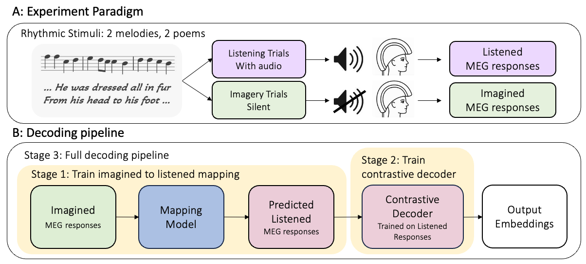
Fig 1: Experiment paradigm and decoding pipeline. (A) Trained musicians were presented with

Fig 2: Imagined-to-listened MEG mapping results. (A) Mean Pearson r between predicted and

Fig 3: Word-level decoding of listened MEG responses using contrastive learning. (A) Overview

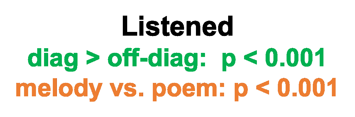
Fig 4: Full pipeline decoding performance and word consistency analysis. (A) Rank CDF for

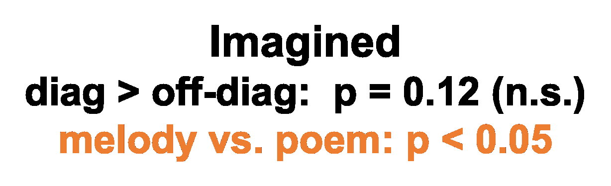
Fig 5 (page 6).

Fig 6 (page 6).

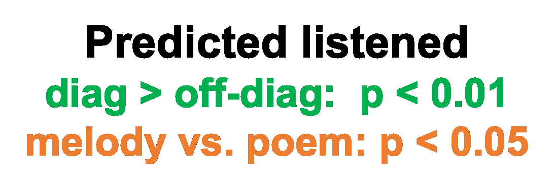
Fig 7 (page 6).

Fig 8 (page 7).

Limitations

• Extremely small and homogeneous subject pool: N=17 trained musicians. Musicians are a highly selected population with superior temporal internalization of rhythmic stimuli; results may not generalize to non-musicians or clinical populations (ALS, LIS) who are the stated target users.
• Vocabulary restricted to 76 content words from two poem excerpts. This is far smaller than real BCI vocabularies and the stimuli are fixed, memorized items rather than novel speech, making the decoding closer to stimulus recognition than open-ended speech decoding.
• No code, weights, or dataset released (as far as can be determined from the truncated text), making independent replication impossible without reproducing the entire MEG collection infrastructure.
• Key training hyperparameters (epochs, batch size, optimizer, learning rate schedule, random seeds) for the neural mapping models and the contrastive decoder are not reported in the main text, relegated to appendices that were truncated.
• The mapping prediction correlations, while significantly above null, are numerically very small (e.g., RNN LOSO mean Pearson r appears to be in the range of 0.01–0.05 based on Fig 2A axis scales), meaning the predicted listened MEG is a noisy approximation; the practical SNR for BCI use remains unclear.
• No adversarial evaluation or robustness testing under distribution shift (e.g., new stimulus types, non-rhythmic speech, different languages, subjects with motor disabilities). The entire experiment uses memorized stimuli, which is a very constrained imagery scenario.
• The listened decoder's train/test split procedure is not fully described in the truncated text — it is unclear whether the decoder was also evaluated in a leave-one-subject-out fashion or trained on all subjects, which would affect the validity of the full pipeline's zero-shot claim.

Open questions / follow-ons

• Does the imagined-to-listened mapping generalize to non-rhythmic, spontaneous imagined speech, or to subjects who are not trained musicians? The temporal alignment advantage of musicians is central to the current design, but BCI target populations (ALS, LIS) cannot be assumed to have musical training.
• Can the mapping be learned from a much smaller number of paired calibration trials per new subject (few-shot personalization), reducing the requirement for full LOSO generalization and improving per-subject decoding accuracy for clinical deployment?
• What is the representational content of the residual error between true listened MEG and predicted listened MEG — does it carry phonetic, prosodic, or identity-specific information, and could a secondary model exploit that residual to improve decoding?
• The transformer mapping model failed due to dataset size limitations — is there a data regime (e.g., via cross-dataset pretraining on listened MEG from larger public corpora) where attention-based global context models outperform recurrent ones for this mapping task?

Why it matters for bot defense

At first glance, imagined speech MEG decoding appears entirely orthogonal to bot defense and CAPTCHA. However, the paper is directly relevant to one emerging threat vector: passive biometric and intent-inference attacks via neural signals. As consumer-grade EEG/BCI headsets (Emotiv, Muse, Meta's neural wristband) become more common, the question of whether passively recorded neural signals can be decoded to infer user intent, cognitive state, or even sub-vocalized responses to CAPTCHA challenges becomes non-trivial. This paper demonstrates a proof-of-concept that even low-SNR, non-invasive MEG signals contain decodable word-level information from imagined speech — a result that, combined with the scalability finding (performance grows monotonically with data), suggests the decoding quality will improve as datasets grow.

For bot-defense engineers, the more immediate takeaway is methodological: the three-stage zero-shot transfer pipeline (rich-domain training → cross-domain mapping → frozen decoder inference) is a general template for exploiting asymmetric data availability, which is exactly the situation adversarial ML researchers face when building bot detectors without labeled bot behavior. The contrastive dual-encoder approach — training on listened MEG, deploying on imagined MEG without retraining — is directly analogous to training a behavior encoder on known-human traffic and deploying it to score unknown sessions. The word consistency analysis (Jaccard similarity of top-K decoded items across subjects and models) is also a useful validation pattern for checking whether a model is detecting real signal versus noise, applicable to consistency checks in bot detection systems.

Cite

@article{arxiv2605_08075,
  title={ Zero-Shot Imagined Speech Decoding via Imagined-to-Listened MEG Mapping },
  author={ Maryam Maghsoudi and Shihab Shamma },
  journal={arXiv preprint arXiv:2605.08075},
  year={ 2026 },
  url={https://arxiv.org/abs/2605.08075}
}

Read the full paper

• arXiv:2605.08075 (abstract)
• arXiv:2605.08075 (PDF)