PET-Adapter: Test-Time Domain Adaptation for Full and Limited-Angle PET Image Reconstruction

Source: arXiv:2605.08030 · Published 2026-05-08 · By Rüveyda Yilmaz, Yuli Wu, Johannes Stegmaier, Volkmar Schulz

TL;DR

PET-Adapter addresses a core practical bottleneck in deep-learning-based PET image reconstruction: models trained on simulation or phantom data degrade substantially when applied to real clinical data with different scanners, tracers, or anatomical populations, and retraining from scratch is infeasible without paired ground-truth clinical measurements. The paper proposes a test-time domain adaptation (TTDA) framework that takes a score-based diffusion model pretrained entirely on BrainWeb phantom data and adapts it—without any paired ground-truth—to target clinical datasets by learning lightweight low-rank conditioning parameters guided by a combined Poisson negative log-likelihood loss and an MRI-driven anatomical TV-weighted loss. Critically, adaptation is performed at the dataset level rather than per-scan, avoiding per-image overfitting and reducing amortized overhead.

The second major contribution is OSEM-based warm-starting: instead of initializing the reverse diffusion chain from pure Gaussian noise (requiring ~50 steps to traverse the full generative trajectory), the authors invert an OSEM reconstruction into a noisy latent state at a fixed noise level (t_r = 0.4) and begin sampling from there. This geometric insight—that OSEM quickly recovers low-frequency anatomy but diverges on high-frequency noise—means the diffusion model only needs to correct high-frequency residuals, reducing required steps from 50 to 2 with no measured quality penalty. The combination of TTDA and warm-starting is evaluated on four heterogeneous clinical PET–MRI brain datasets (CERMEP, AGIEF, NeuroExplorer/NX, Huntington mouse models) in both full-angle and limited-angle (40% detectors disabled) settings.

Results in Table 1 show consistent and large PSNR/SSIM gains over five baselines (OSEM, Bowsher, PET-PIR, PET-DDS, LiSch-SCD), with the proposed method using only T=2 diffusion steps versus T=50 for all competing diffusion approaches. Ablation in Table 2 confirms both warm-starting and TTDA are individually necessary: removing either one causes 3–9 dB PSNR drops depending on dataset and angle setting.

Key findings

• PET-Adapter at T=2 diffusion steps achieves PSNR of 35.3/35.4/37.6/30.7 dB (SSIM 0.96/0.96/0.95/0.91) on CERMEP/AGIEF/NX/Huntington in the full-angle setting, compared to the next-best diffusion baseline LiSch-SCD at T=50 achieving 32.7/29.4/35.7/28.3 dB (Table 1a).
• In the limited-angle setting, PET-Adapter (T=2) reaches 32.2/31.7/32.0/25.2 dB PSNR vs LiSch-SCD (T=50) at 26.4/27.3/30.9/23.4 dB across the four datasets (Table 1b), a gain of up to 5.8 dB on CERMEP.
• Warm-starting reduces required diffusion steps from 50 to 2: ablation shows that without WS at T=2 the model drops to 29.6/29.1/30.9/26.7 dB (FA), recovering to 34.9/36.4/35.2/31.2 dB only when T is restored to 50 (Table 2a).
• Removing TTDA while retaining WS at T=2 causes PSNR to fall to 26.2/26.3/34.7/24.7 dB (FA) and 21.8/23.3/28.3/20.6 dB (LA), confirming that phantom-to-clinical domain gap is the primary performance limiter and adaptation is not cosmetic (Table 2b).
• The same pretrained score model weights are shared for both full-angle and limited-angle experiments; only the sinogram loss mask changes for LA, demonstrating geometry-agnostic adaptation.
• Warm-starting inversion is set to t_r = 0.4 (40% of the diffusion trajectory), chosen based on the geometric argument that OSEM reconstructions lie close to the low-frequency manifold but are not clean images; this hyperparameter is not ablated across values in the paper.
• The TTDA hyperparameters (λ, σ, rank r, learning rate) are set using only two held-out samples from each target dataset, suggesting the adaptation is not data-hungry.
• Dataset-level global adaptation is used rather than per-scan adaptation, explicitly contrasting with per-image approaches of Hashimoto et al. and Webber et al., which the authors argue risks per-image overfitting.

Threat model

n/a — this is a medical imaging reconstruction paper, not a security paper. The 'adversarial' framing here is distributional: the model pretrained on BrainWeb phantom data encounters out-of-distribution clinical data at test time. The adversary is statistical distribution shift (different scanner hardware, tracer chemistry, pathological anatomy, species), not an intentional attacker. The method assumes the system matrix A and background b are known or estimable, and that co-registered MR images are available at test time. It explicitly cannot handle absence of MR guidance or completely unknown PET physics.

Methodology — deep read

Threat model and assumptions (domain shift framing): The adversarial distribution shift here is the phantom-to-clinical gap: the pretrained score model sθ has seen only BrainWeb simulated FDG-PET brain phantoms (20 volumes, 2D slices). At test time it must generalize to four unseen clinical distributions—healthy adult brains (CERMEP), epilepsy patients with focal hypometabolism (AGIEF), multi-tracer long-axial-FOV scanner data (NX), and mouse Huntington's disease models. The key assumption is that paired ground-truth clinical PET is unavailable for adaptation; only raw sinogram measurements y and co-registered MR images are accessible. The model also assumes the PET physics model (system matrix A, background b) is known well enough to compute a Poisson NLL loss.

Data provenance, size, and preprocessing: Training uses BrainWeb (20 simulated FDG-PET volumes with coregistered MR, 2D slice extraction). For CERMEP and AGIEF, GT reference volumes are constructed by averaging PET intensities within MRI-segmented brain regions to produce high-SNR pseudo-GT (since native acquisition quality is described as low). NX provides directly acquired high-quality multi-tracer PET/CT data with paired MR. Huntington data uses mouse MRI from the Cambridge database with simulated [18F]FDG uptake assigned to segmented gray/white matter. PET measurements for all datasets are simulated from GT using Parallelproj, with true counts per emission volume set to 10; limited-angle simulations disable 40% of detectors. Image-wise normalization sets the mean emission value of each training image to 1.0. TTDA hyperparameters are tuned on 2 held-out samples per target dataset. Train/test split details beyond this are not explicitly stated.

Architecture and novel components: The base model sθ is a U-Net-based score function (from Singh et al., PET-DDS [21]), trained with denoising score matching loss L_DSM. Inference uses a generalized DDIM/variance-preserving SDE update (Eq. 2) with Tweedie's estimate ˆx₀ and data-consistency via MAP update (preconditioned gradient ascent with EM preconditioner on Poisson log-likelihood). The novel module is the layer-wise low-rank anatomical conditioning block (Eq. 3, Fig. 1c): for each U-Net convolutional layer l with frozen weight W₀, a low-rank delta ΔW = U·D(x_l | g(x_MR)) is added, where D ∈ R^{r×k} and U ∈ R^{d×r} are learnable with rank r ≪ min(d,k), and a mapper g projects x_MR into a latent space from which FiLM-style scale γ_φ and shift β_φ parameters are produced. This is an application of CTRLorALTer-style conditional LoRA [24] to medical imaging. Inputs are the layer activations x_l and the MR image x_MR; output is an MR-modulated layer activation h_l. Only the adaptation parameters (D, U, g, γ_φ, β_φ) are trained during TTDA; W₀ is frozen.

Adaptation objective: L_adapt = L_p + λ·L_a. L_p is the Poisson NLL between measured prompts y and forward projection ŷ = A·ˆx_MAP + b. L_a is an MRI-guided anatomical smoothness loss: edge-weighted TV where weights w_j = exp(−‖∇x_MR‖_j / σ) penalize gradients more in homogeneous tissue regions and less at anatomical boundaries (Eq. 4). For LA, sinogram regions corresponding to missing detectors are masked out of L_p. λ and σ are hyperparameters set from 2 held-out samples.

Warm-starting mechanism: Classical MLEM/OSEM theory (Zeng [34]) establishes that large singular-value (low-frequency) components converge in early iterations while prolonged iteration fits Poisson noise. The authors use this to argue that a moderate-iteration OSEM reconstruction (30 subsets, 2 iterations—matching intensity normalization requirements already needed for inference) is geometrically close to the clean image manifold in low-frequency components but noisy otherwise. Warm-starting inverts the OSEM image into a noisy diffusion latent at t_r = 0.4 via DDIM inversion [9,22,33], then begins the reverse SDE from that point rather than from pure Gaussian noise. This bypasses the ~48 low-frequency generation steps, leaving only 2 residual refinement+data-consistency iterations needed. The OSEM images are not extra overhead since they are already required for intensity normalization (as in Singh et al. and Webber et al.). A concrete end-to-end inference pass: (1) Compute OSEM reconstruction ˆx_MAP from y using 30 subsets, 2 iterations; (2) normalize ˆx_MAP; (3) invert via forward DDIM to obtain x_{t_r} at t_r=0.4; (4) run T=2 alternating reverse-SDE steps (prior refinement via sθ → Tweedie estimate ˆx₀ → MAP data-consistency update); (5) denormalize output.

Training regime: sθ is trained on 2D slices from 3D BrainWeb volumes (not 3D volumes directly, due to limited training data). Training: 2000 epochs, batch size 32, learning rate 1×10⁻⁴, NVIDIA RTX 4000 GPU. No seed strategy or data augmentation details are reported. The same model is used for both FA and LA (the score prior is geometry-independent). TTDA training details (number of adaptation steps, learning rate for adaptation, rank r) are not explicitly stated in the provided text—this is a reproducibility gap.

Evaluation protocol: Metrics are PSNR and SSIM on 3D reconstructed volumes evaluated against the GT references. Five baselines are compared: OSEM, MAPEM-Bowsher (MR-guided classical), PET-PIR (DiffPIR + feature injection + MR + PET updates), PET-DDS (Singh et al., CFG-guided score model), LiSch-SCD (Webber et al., Steerable Conditional Diffusion). All diffusion baselines use T=50. LiSch-SCD was reimplemented by the authors as the original code is not public. No statistical significance tests (confidence intervals, paired t-tests) are reported. No cross-validation; test splits are not quantified in subject count. Ablation covers WS and TTDA removal, with two T configurations (2 and 50) for the no-WS case.

Technical innovations

• Layer-wise conditional LoRA adaptation of a frozen diffusion score function using FiLM-style MR-derived scale/shift parameters (CTRLorALTer [24] extended to PET reconstruction), enabling anatomy-guided test-time adaptation without any paired PET ground truth.
• OSEM warm-starting via DDIM inversion at t_r=0.4, exploiting the spectral convergence property of iterative EM algorithms to reduce diffusion sampling from 50 to 2 steps without quality loss—distinct from prior per-scan DIP-based inversion approaches [5,28].
• Dataset-level (rather than per-image) TTDA for PET reconstruction, contrasting with per-scan adaptation in Hashimoto et al. [5] and Webber et al. [28], reducing overfitting risk and amortizing adaptation cost across a full clinical cohort.
• TV-weighted MRI anatomical loss (Eq. 4) that spatially modulates gradient penalties based on MR edge magnitude, encouraging homogeneous-region smoothness while preserving anatomical boundaries during adaptation.
• Unified full-angle and limited-angle reconstruction under a single pretrained model by masking missing sinogram contributions in L_p during LA adaptation, without any LA-specific architectural changes.

Datasets

• BrainWeb — 20 simulated FDG-PET volumes with coregistered MR — publicly available phantom dataset (Aubert-Broche et al. 2006)
• CERMEP-IDB-MRXFDG — 37 healthy adult [18F]FDG PET + T1/FLAIR MRI + CT — CERMEP / Hospices Civils de Lyon (partially restricted; acknowledgement required)
• AGIEF — unspecified number of subjects including healthy and epilepsy patients, multi-tracer PET+MRI — Zhang et al. 2022 (non-public, institutional)
• NeuroExplorer (NX) — multi-tracer long-axial-FOV PET/CT + MRI — Volpi et al. 2025 (non-public, institutional)
• Cambridge Huntington's Disease Mouse MRI Database — mouse brain MRI with simulated [18F]FDG PET — Sawiak & Morton 2016 (publicly available)

Baselines vs proposed

• OSEM (FA): PSNR=29.2/28.9/30.7/26.7, SSIM=0.85/0.82/0.89/0.88 vs Ours: PSNR=35.3/35.4/37.6/30.7, SSIM=0.96/0.96/0.95/0.91 (CERMEP/AGIEF/NX/Huntington)
• MAPEM-Bowsher (FA): PSNR=30.4/29.5/32.1/28.0, SSIM=0.89/0.83/0.94/0.90 vs Ours: PSNR=35.3/35.4/37.6/30.7, SSIM=0.96/0.96/0.95/0.91
• PET-PIR T=50 (FA): PSNR=24.5/27.2/36.4/25.5, SSIM=0.84/0.77/0.96/0.84 vs Ours T=2: PSNR=35.3/35.4/37.6/30.7, SSIM=0.96/0.96/0.95/0.91
• PET-DDS T=50 (FA): PSNR=27.4/32.1/35.7/24.9, SSIM=0.83/0.91/0.94/0.81 vs Ours T=2: PSNR=35.3/35.4/37.6/30.7, SSIM=0.96/0.96/0.95/0.91
• LiSch-SCD T=50 (FA): PSNR=32.7/29.4/35.7/28.3, SSIM=0.92/0.85/0.95/0.87 vs Ours T=2: PSNR=35.3/35.4/37.6/30.7, SSIM=0.96/0.96/0.95/0.91
• OSEM (LA): PSNR=25.5/24.9/23.8/25.0, SSIM=0.74/0.69/0.67/0.75 vs Ours: PSNR=32.2/31.7/32.0/25.2, SSIM=0.91/0.87/0.92/0.78
• LiSch-SCD T=50 (LA): PSNR=26.4/27.3/30.9/23.4, SSIM=0.81/0.78/0.90/0.70 vs Ours T=2: PSNR=32.2/31.7/32.0/25.2, SSIM=0.91/0.87/0.92/0.78
• Ablation w/o WS T=2 (FA): PSNR=29.6/29.1/30.9/26.7, SSIM=0.85/0.84/0.90/0.79 vs full PET-Adapter T=2: PSNR=35.3/35.4/37.6/30.7, SSIM=0.96/0.96/0.95/0.91
• Ablation w/o TTDA T=2 (FA): PSNR=26.2/26.3/34.7/24.7, SSIM=0.74/0.73/0.91/0.78 vs full PET-Adapter T=2: PSNR=35.3/35.4/37.6/30.7, SSIM=0.96/0.96/0.95/0.91

Figures from the paper

Figures are reproduced from the source paper for academic discussion. Original copyright: the paper authors. See arXiv:2605.08030.

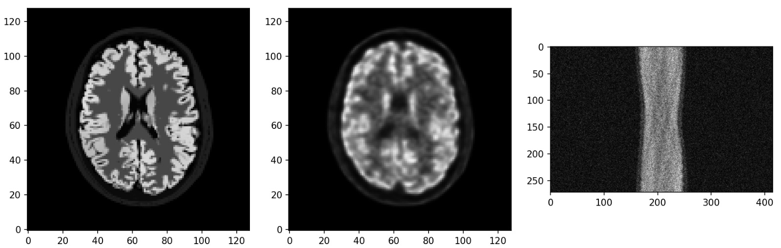
Fig 1: The architecture of PET-Adapter. (a) Pretraining on phantom data is

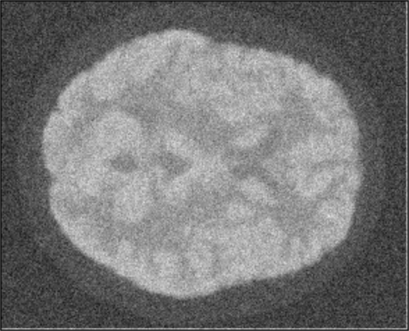
Fig 2 (page 3).

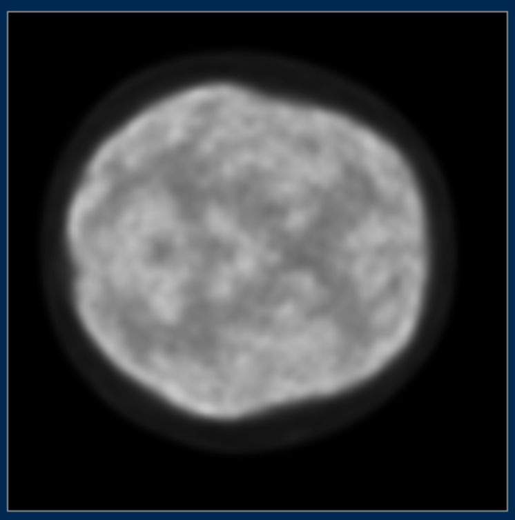
Fig 3 (page 3).

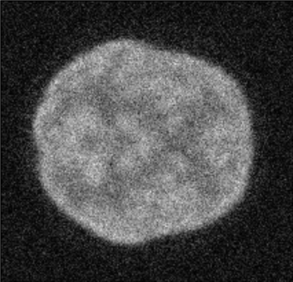
Fig 4 (page 3).

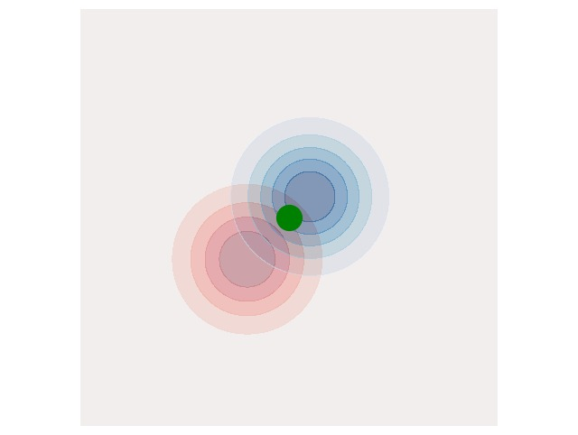
Fig 5 (page 3).

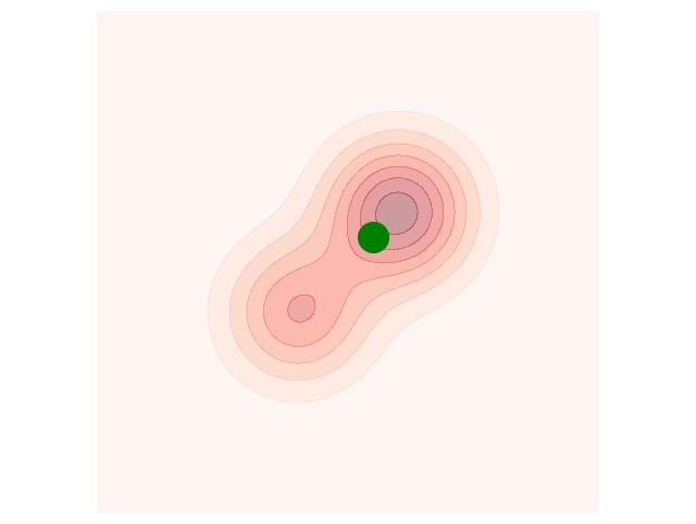
Fig 6 (page 3).

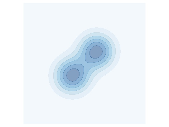
Fig 7 (page 3).

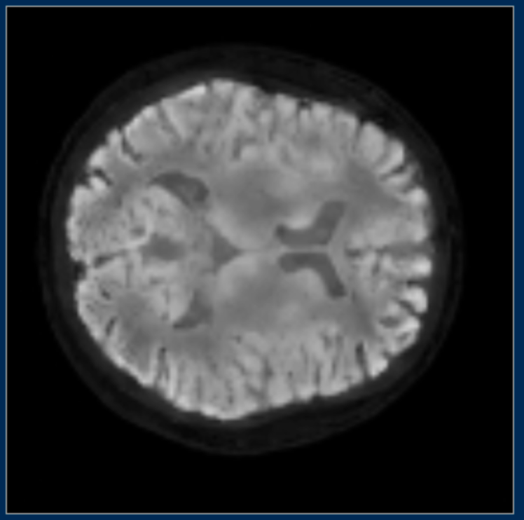
Fig 8 (page 3).

Limitations

• No statistical significance testing: all PSNR/SSIM comparisons are point estimates with no confidence intervals, paired t-tests, or bootstrap resampling, making it impossible to assess whether differences (especially small ones like NX FA: 37.6 vs PET-PIR 36.4 dB) are reliable.
• Dataset sizes are small and not fully reported: the number of test subjects per dataset is never stated; CERMEP has 37 subjects total but how many are used for test is unclear, and Huntington uses simulated PET on mouse data which may not generalize to clinical neurodegeneration cases.
• Key TTDA hyperparameters (rank r, number of adaptation gradient steps, adaptation learning rate, λ, σ) are set from only 2 held-out samples per dataset and not ablated systematically—sensitivity to these choices is unknown.
• LiSch-SCD (Webber et al.) was reimplemented by the authors rather than run from released code, introducing a potential reimplementation gap that could disadvantage this baseline unfairly.
• The model is trained on 2D slices despite operating in a 3D reconstruction setting; inter-slice consistency is handled only implicitly through OSEM warm-starting. No formal analysis of z-direction artifact propagation or slice-inconsistency is provided.
• Warm-starting inversion level t_r = 0.4 is a fixed choice with no ablation across values; the sensitivity of step-count reduction to this hyperparameter (e.g., would t_r=0.3 allow T=1 or degrade quality at T=2?) is unexamined.
• No runtime/wall-clock comparison is reported for the adaptation phase itself (only the inference step count is reduced); the cost of learning the LoRA adaptation parameters per new dataset is not quantified.

Open questions / follow-ons

• How sensitive is the T=2 step reduction to the warm-starting inversion level t_r? Would a systematic sweep (t_r ∈ {0.2, 0.3, 0.4, 0.5, 0.6}) reveal a quality–speed Pareto frontier, and could T=1 be achieved without regression on harder datasets like Huntington?
• The adaptation uses only 2 held-out samples per target dataset for hyperparameter selection—how much does performance degrade as this number approaches 0 (zero-shot TTDA), and is there a principled way to set λ and σ without any target samples?
• The method is validated exclusively on brain PET; PET reconstruction for oncology (whole-body, lesion heterogeneity, respiratory motion) involves very different spatial statistics and scanner geometries—would the same LoRA conditioning architecture transfer, or would the rank and conditioning design need rethinking?
• Dataset-level adaptation assumes a coherent target cohort; in practice a hospital deployment sees a continuous stream of scans from varying protocols. How would an online or continual adaptation scheme avoid catastrophic forgetting of previously adapted distributions while handling single-scan inference pressure?

Why it matters for bot defense

At first glance, PET reconstruction has no direct connection to bot defense or CAPTCHA systems. However, the underlying methodological problem—a model trained in a controlled synthetic environment (phantom data) that must generalize to adversarially diverse real-world distributions (clinical scanners, novel tracers, pathologies) without retraining or ground-truth labels—is structurally identical to a core challenge in bot detection: a classifier trained on known bot signatures must adapt to novel bot populations (new user agents, behavioral drift, adversarial script updates) without labeled examples of the new threat and without breaking legitimate user experience. The TTDA framework's use of unsupervised loss signals (measurement fidelity + structural regularization from a side channel, analogous to sinogram + MRI) maps conceptually onto bot defense scenarios where traffic logs provide implicit signal and device fingerprints or behavioral signals provide structural priors.

More concretely, the warm-starting insight—that a physics-based approximate solution (OSEM) can anchor a generative model so it only needs to correct residuals—is analogous to using heuristic rule-based bot classifiers to warm-initialize a learned model, reducing the effective search space and inference cost. The low-rank LoRA-style conditional adaptation also offers a template for lightweight domain adaptation of large pretrained bot-detection models to site-specific traffic distributions without full retraining, using only a handful of representative unlabeled samples. A bot-defense engineer should note the paper's honest acknowledgment that only 2 calibration samples per target domain were used—this matches the realistic constraint of limited labeled data in new deployment contexts, and the approach is worth evaluating in that framing even if the specific PET architecture is irrelevant.

Cite

@article{arxiv2605_08030,
  title={ PET-Adapter: Test-Time Domain Adaptation for Full and Limited-Angle PET Image Reconstruction },
  author={ Rüveyda Yilmaz and Yuli Wu and Johannes Stegmaier and Volkmar Schulz },
  journal={arXiv preprint arXiv:2605.08030},
  year={ 2026 },
  url={https://arxiv.org/abs/2605.08030}
}

Read the full paper

• arXiv:2605.08030 (abstract)
• arXiv:2605.08030 (PDF)