GRAPHLCP: Structure-Aware Localized Conformal Prediction on Graphs

Source: arXiv:2605.08074 · Published 2026-05-08 · By Peyman Baghershahi, Fangxin Wang, Debmalya Mandal, Sourav Medya

TL;DR

GRAPHLCP addresses the problem of uncertainty quantification for graph neural networks (GNNs) using conformal prediction (CP). Standard CP assumes exchangeable (i.i.d.) samples and relies on proximity in embedding space for localization, but GNN embeddings suffer from over-smoothing, over-squashing, and under-confidence, making embedding-based similarity measures unreliable or non-discriminative. Existing graph CP methods either depend on pure embedding-space kernels or hard structural clustering, both of which degrade under heterophily or sparse topologies.

GRAPHLCP replaces embedding-only proximity with a Personalized PageRank (PPR)-based localization kernel that captures soft, multi-hop structural proximity. Before applying PPR, the authors introduce a feature-aware graph densification step: PCA is used to decorrelate and compress GNN embeddings, then an anisotropic Gaussian kernel with PCA-eigenvalue-derived bandwidths is used to add high-confidence embedding-similarity edges to the graph, bridging sparse regions. This densified graph is then used for PPR computation, anchor sampling, and calibration weighting in the Randomly Localized Conformal Prediction (RLCP) framework.

Experiments span seven node regression datasets and six node classification datasets against six baselines. GRAPHLCP achieves marginal coverage at the target level (alpha=0.1) across all datasets, and demonstrates best or second-best worst-slab coverage (WSC) conditional coverage while producing tighter prediction sets than the strongest localized baseline (CalLCP). The PPR kernel is ablated against a Gaussian embedding-space kernel, confirming structure-aware localization as the primary driver of improvement.

Key findings

• GRAPHLCP achieves marginal coverage at or above 1-alpha=0.9 across all 13 tested datasets (7 regression, 6 classification), as shown in Table 1, confirming conformal validity is preserved under the transductive GNN setup.
• On worst-slab coverage (WSC), evaluated over 100 random direction vectors on the unit sphere, GRAPHLCP achieves best or second-best results across most of the 13 datasets in Figure 2, outperforming SCP, RLCP, CF-GNN, SNAPS, and often CalLCP on classification datasets.
• GRAPHLCP outperforms CalLCP in normalized prediction length (efficiency) across datasets (Figure 3), even when CalLCP achieves slightly higher WSC, making GRAPHLCP's prediction sets more compact on average.
• PPR kernel ablation (Table 2) shows PPR consistently achieves higher WSC coverage than an embedding-space Gaussian kernel (GSS) on 9 of 10 datasets (e.g., CBAS: PPR 0.64±.03 vs GSS 0.52±.06) while also yielding tighter or comparable prediction lengths on most datasets.
• The densification step is identified as the largest single contributor in component ablation (Table 3, %NI metric), particularly on regression datasets (ANH, CHI, TWT), with PCA projection as the second most impactful component.
• CalLCP exceeded a 3-day time limit on large classification graphs (CMP, DBLP), while GRAPHLCP completed within acceptable time, demonstrating a scalability advantage on large-graph settings.
• NAPS produces infinite-length prediction intervals (-) on all seven regression datasets (Table 1), rendering it inapplicable for regression tasks in this benchmark.
• Group-based conditional coverage partitioned by homophily and feature clustering (Figure 4) consistently shows GRAPHLCP's superiority over CF-GNN and SCP on CHI, INC, UNM, and TWT datasets, with minimum partition coverage approaching or exceeding 0.9 more reliably than baselines.

Threat model

n/a — This is not a security paper in the adversarial-ML sense. The paper focuses on uncertainty quantification (conformal prediction) for GNNs. The closest analog to a threat model is the worst-slab coverage (WSC) evaluation, which acts as an implicit adversarial diagnostic: it searches over 100 random unit-sphere projection directions to identify the subpopulation of test nodes with minimum coverage, stress-testing whether the method's conditional coverage holds in the worst-case subgroup. No explicit attacker capabilities, knowledge assumptions, or attack scenarios are defined.

Methodology — deep read

THREAT MODEL AND ASSUMPTIONS: This is not a security paper in the adversarial-ML sense. The 'adversary' in the CP context is an implicit one: the worst-slab coverage (WSC) evaluation adversarially searches over 100 random projection directions on the unit sphere to find the bounded interval of the feature space where coverage is minimized. The authors assume a transductive node-level setting where the GNN is trained on Dtr, calibration nodes Dcal have labels held out from training, and test nodes Dtest are unlabeled. Because GNN operations are permutation-equivariant and nonconformity scores are permutation-invariant over calibration and test node permutations, standard marginal CP coverage guarantees hold under this setup (following [18, 27]). Node dependence is managed by operating in the transductive regime with random splits, preserving exchangeability between calibration and test nodes.

DATA: The paper evaluates on 7 node regression datasets (ANH, CHI, EDU, ELC, INC, UNM, TWT) and 6 node classification datasets (CMP, CRA, DBLP, CBAS, WKB, PMD). Dataset details and statistics are deferred to Appendix A.10, which is not fully reproduced in the truncated text. Splits are train/calibration/test with the calibration set providing labeled holdout data for conformal quantile computation. The miscoverage rate alpha is fixed at 0.1 across all experiments. No further detail on split ratios, seeds, or label distributions is available in the provided text.

ARCHITECTURE AND ALGORITHM: GRAPHLCP is a post-hoc wrapper around a frozen pretrained GNN; it does not modify GNN training. The pipeline has four stages. (1) PCA Transformation: calibration embeddings (last-layer GNN representations) are centered and PCA is applied to compute the covariance matrix CX = (1/n) * X_cal^T * X_cal. The top-c eigenvectors form Vc, projecting embeddings to a lower-dimensional space zi = Vc^T xi. This decorrelates features and concentrates variance, counteracting over-smoothing which collapses high-frequency variation. (2) Graph Densification: an anisotropic Gaussian kernel with adaptive bandwidth is computed in the PCA-reduced space using the Mahalanobis distance H(x,x';h^2Lambda_c) = exp(-0.5 * DM^2(x,x';h^2Lambda_c)), where bandwidths per dimension are proportional to the PCA eigenvalues. Edges are added to the adjacency matrix wherever kernel similarity exceeds an automatically determined threshold tau_d (derived from empirical homophily analysis, Appendix A.5). The densification is applied uniformly across all nodes before any split-dependent operations, preserving calibration-test symmetry. (3) PPR Integration: PPR is computed on the densified graph using power iteration with K=30 steps and restart probability beta. For a test node u_{n+1}, the anchor node is sampled from the PPR distribution pi_{n+1} (a two-step process: sample walk length k ~ Geom(beta), then follow a k-step random walk from u_{n+1}, capped at K steps). Calibration and test nodes are weighted by their structural proximity to the anchor using the degree-normalized symmetry property of PPR: w_i ~ d_i^{-1} * [pi_tilde]i, normalized over all n+1 samples. This avoids computing all n PPR vectors when n > m test samples by exploiting undirected graph symmetry. (4) Conformal Prediction: weighted quantile q is computed over calibration nonconformity scores using weights from step 3, following the RLCP formulation. Prediction sets are {y: s(x_{n+1}, y) <= q_{1-alpha}(x_{n+1}, x_tilde_{n+1})}.

TRAINING REGIME: The GNN base model is pretrained and then frozen; GRAPHLCP adds no learnable parameters. The PPR computation uses K=30 power iterations. The PCA dimensionality c and base bandwidth h are hyperparameters; the densification threshold tau_d is set automatically via a homophily-guided heuristic (Appendix A.5). Specific values of c, h, random seeds, and hardware are not detailed in the provided truncated text.

EVALUATION PROTOCOL: Three evaluation axes are used. (1) Marginal coverage (Table 1): sanity check that all methods achieve >= 1-alpha = 0.9 coverage. (2) Worst-slab coverage (WSC, Figure 2 and Figure 3): an adversarial metric that searches 100 random unit-sphere direction vectors and finds the projection slab with minimum coverage, representing the hardest subpopulation. (3) Group-based conditional coverage (Figure 4): test nodes are partitioned into three equal quantile bins ('Low', 'Mid', 'High') based on four features—clustering coefficient, feature clustering (embedding-based), homophily, and node degree. Minimum coverage across partitions is reported. Baselines include SCP (vanilla split CP), RLCP, CalLCP (localized CP methods), and NAPS, CF-GNN, SNAPS (graph-specific CP methods). Prediction interval efficiency (normalized length/size) is reported alongside coverage in Figure 3. No statistical significance tests or confidence intervals beyond standard deviation across runs are reported. Cross-validation details are not stated. CalLCP is excluded from large graph results due to out-of-time (>3 days) computation.

CONCRETE EXAMPLE END-TO-END: Consider a test node u_{n+1} in a sparse social network (e.g., TWT dataset). (i) The frozen GNN produces a 128-dim embedding for u_{n+1}. (ii) PCA reduces calibration embeddings to c dimensions, retaining top eigenvalue directions; u_{n+1}'s embedding is projected similarly. (iii) The anisotropic Gaussian kernel is computed between all node pairs in PCA space; pairs exceeding tau_d receive new edges in the densified adjacency matrix A_tilde. (iv) PPR is run on A_tilde for u_{n+1} as seed, yielding pi_{n+1} over all nodes. A walk length k ~ Geom(beta) is sampled, and a k-step random walk yields anchor node u_tilde_{n+1}. (v) Calibration weights w_i are computed as degree-normalized PPR scores from u_tilde_{n+1}. (vi) Weighted quantile q_{0.9} is computed from calibration nonconformity scores. (vii) The prediction set for u_{n+1} is all labels y with nonconformity score <= q_{0.9}.

REPRODUCIBILITY: Pseudocode is provided in Appendix A.4 (Algorithm 1). No code repository or frozen weights release is mentioned in the provided text. Several implementation details (exact PCA dimension c, bandwidth h, beta, split ratios, hardware) are either in appendices not fully reproduced or not stated, which limits reproducibility from the main paper alone.

Technical innovations

• PPR as a localization kernel for conformal prediction on graphs: instead of using embedding-space Gaussian kernels (as in RLCP [16]) or hard community-based clustering (as in [46]), GRAPHLCP uses Personalized PageRank on the (densified) graph to define soft, multi-hop, direction-dependent structural proximity for both anchor sampling and calibration weighting.
• Feature-aware graph densification prior to PPR: a novel preprocessing step that augments the sparse graph adjacency with high-confidence embedding-similarity edges (selected via an anisotropic Gaussian kernel in PCA-reduced space), preventing PPR's probability mass from collapsing locally in sparse graphs and bridging heterophilic regions.
• Anisotropic, eigenvalue-adaptive Gaussian kernel for edge selection: bandwidths per PCA dimension are set proportional to PCA eigenvalues, capturing non-uniform embedding geometry caused by GNN over-smoothing, distinguishing it from isotropic kernel approaches used in prior localized CP work.
• Degree-normalized PPR symmetry exploitation for efficient weighting: for undirected graphs, the authors exploit d_i * H(u_i, u_j) = d_j * H(u_j, u_i) to avoid computing all n calibration-node PPR vectors when n > m test samples, reducing computational cost compared to a naive n-PPR-vector approach.
• Homophily-guided automatic densification threshold: the threshold tau_d controlling how many new edges are added is set automatically based on empirically observed correlation between node homophily and coverage quality (Appendix A.3, A.5), rather than requiring manual tuning per graph.

Datasets

• ANH — size not specified in provided text — source not specified (node regression)
• CHI — size not specified in provided text — source not specified (node regression)
• EDU — size not specified in provided text — source not specified (node regression)
• ELC — size not specified in provided text — source not specified (node regression)
• INC — size not specified in provided text — source not specified (node regression)
• UNM — size not specified in provided text — source not specified (node regression)
• TWT — size not specified in provided text — source not specified (node regression)
• CMP — size not specified in provided text — source not specified (node classification)
• CRA — size not specified in provided text — source not specified (node classification)
• DBLP — size not specified in provided text — source not specified (node classification)
• CBAS — size not specified in provided text — source not specified (node classification)
• WKB — size not specified in provided text — source not specified (node classification)
• PMD — size not specified in provided text — source not specified (node classification)

Baselines vs proposed

• SCP (vanilla split CP): marginal coverage ~0.900-0.905 across all 13 datasets; WSC conditional coverage generally lowest among methods (Fig 2); prediction sets valid but not locally adapted
• RLCP [16]: marginal coverage ~0.895-0.904 across datasets (Table 1); WSC coverage competitive with SCP but below GRAPHLCP on most datasets (Fig 2); authors note embedding collapse causes proximity weights to degenerate
• CalLCP [14]: marginal coverage 0.907-0.943 on available datasets (OOT on CMP and DBLP); WSC sometimes best among baselines on regression datasets but GRAPHLCP achieves comparable or better WSC with strictly smaller normalized prediction length (Fig 3)
• CF-GNN [18]: marginal coverage 0.898-0.920 across datasets (Table 1); WSC coverage generally below GRAPHLCP (Fig 2, Fig 4)
• SNAPS [40]: marginal coverage 0.896-0.969 across datasets, produces infinite intervals on TWT regression (Table 1)
• NAPS [7]: produces infinite-length prediction intervals on all 7 regression datasets (Table 1); marginal coverage 0.934-1.000 on classification datasets but with inflated prediction sets
• GRAPHLCP (proposed): marginal coverage 0.897-0.917 across all 13 datasets (Table 1); best or second-best WSC on most datasets (Fig 2); second-best overall WSC but best normalized prediction length vs CalLCP (Fig 3); PPR variant WSC coverage 0.60-0.76 vs GSS variant 0.52-0.72 across 10 datasets (Table 2)

Figures from the paper

Figures are reproduced from the source paper for academic discussion. Original copyright: the paper authors. See arXiv:2605.08074.

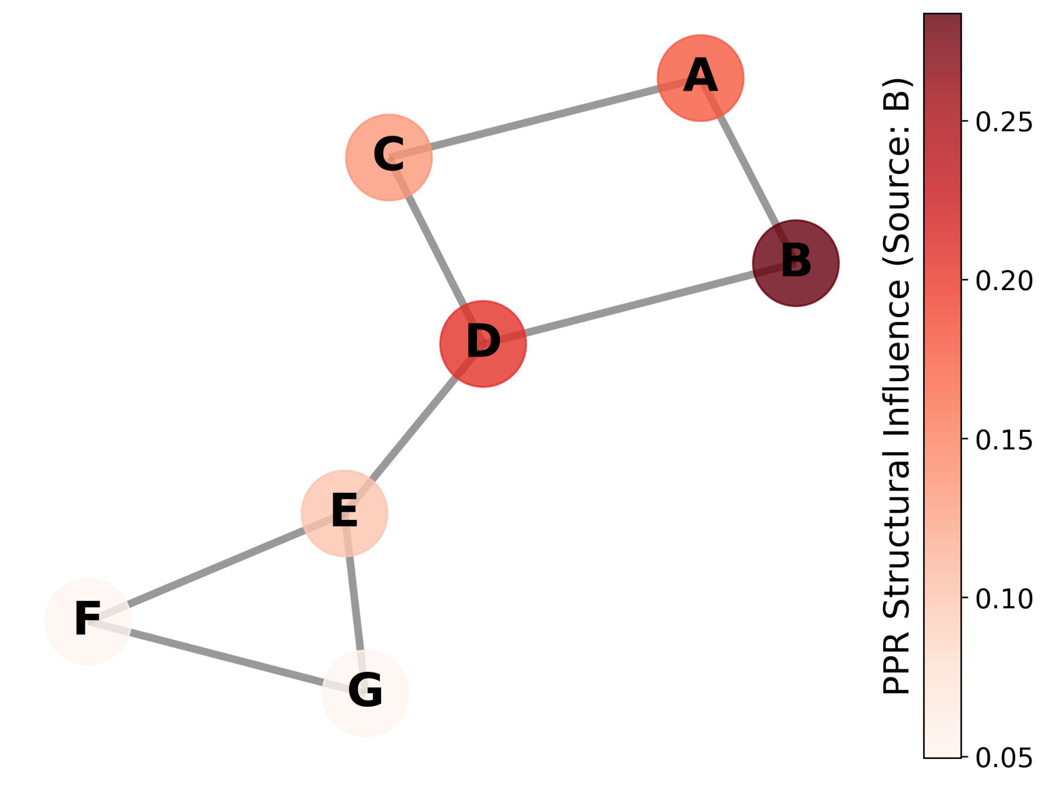
Fig 1: GRAPHLCP. Given the embeddings of a frozen GNN for an input graph, GRAPHLCP goes

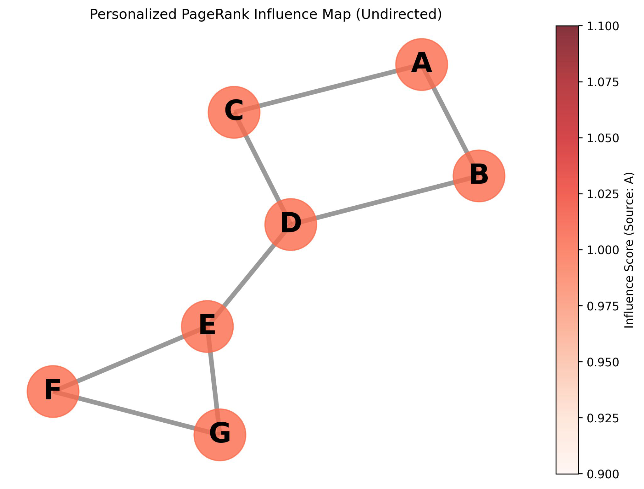
Fig 2 (page 4).

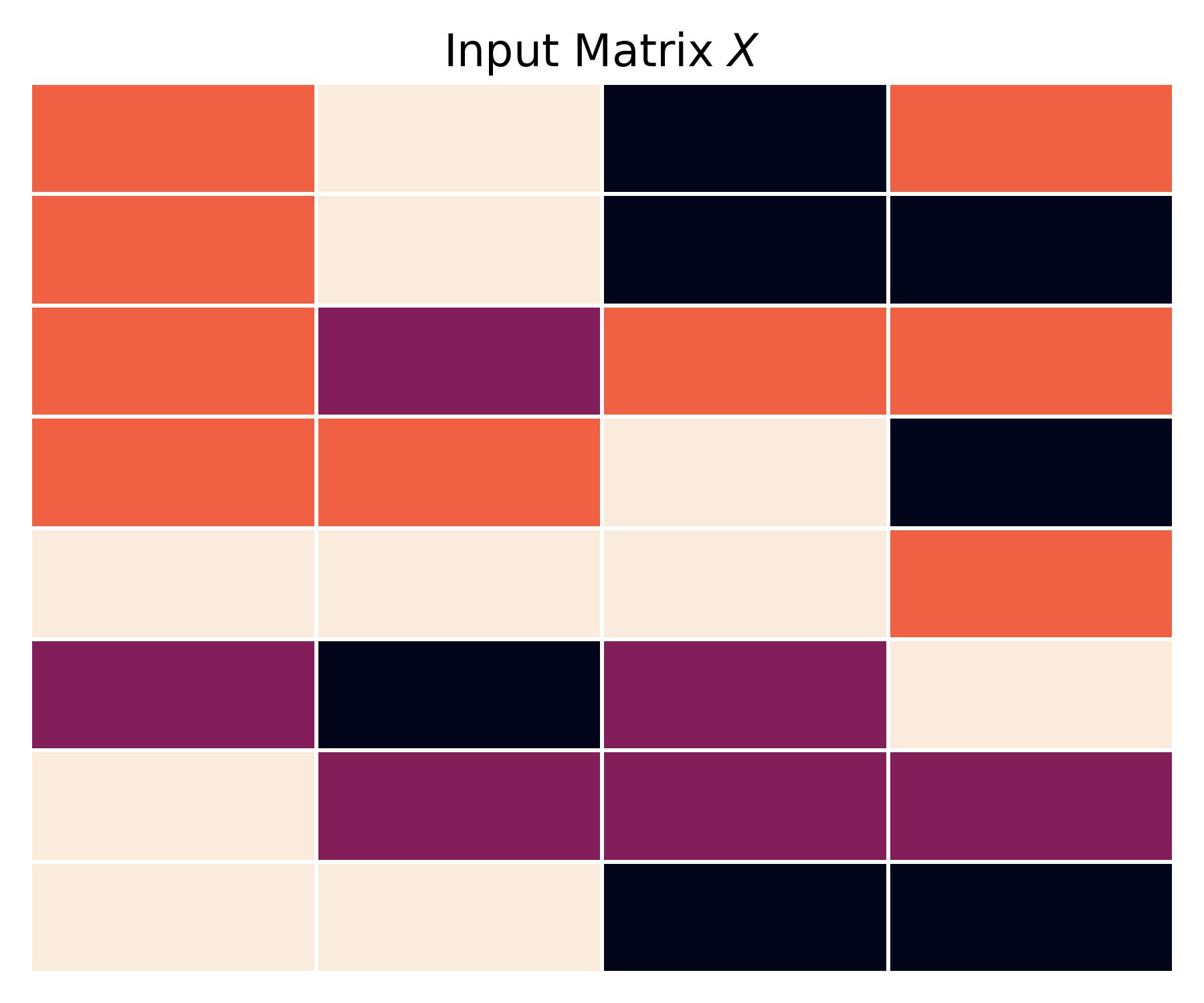
Fig 3 (page 4).

Fig 4 (page 4).

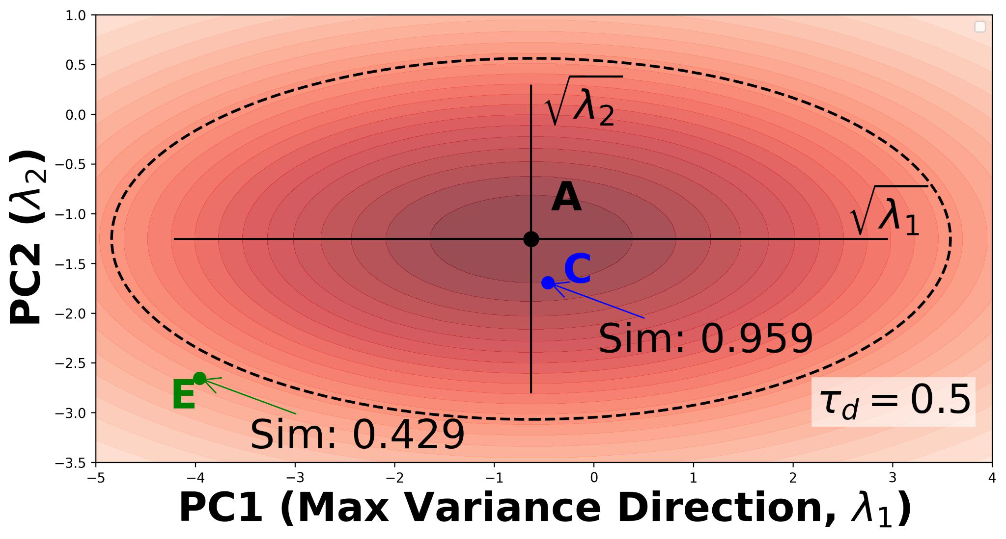
Fig 5 (page 4).

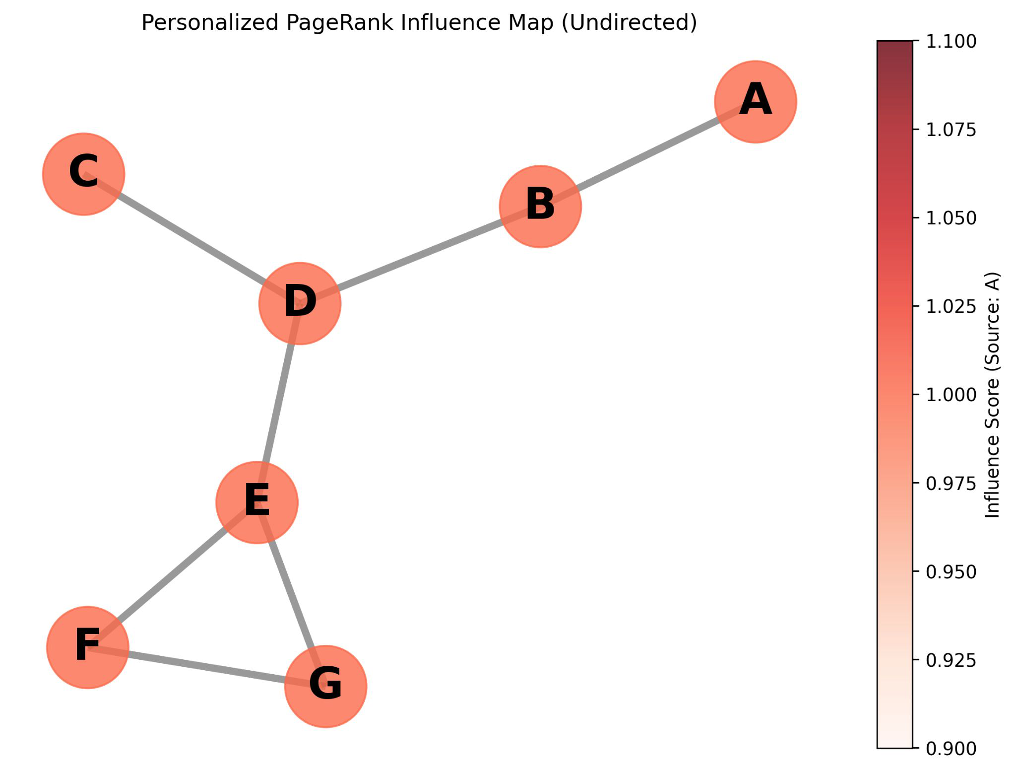
Fig 6 (page 4).

Limitations

• Dataset and split details (sizes, split ratios, label distributions, random seeds) are deferred entirely to Appendix A.10 and A.6, which are not provided; this makes it impossible to fully assess generalizability or reproduce results from the main paper text alone.
• No code repository or model weights release is mentioned; with several hyperparameters (PCA dimension c, bandwidth h, restart probability beta, densification threshold tau_d) and their selection criteria spread across appendices, reproducibility is uncertain.
• The automatic densification threshold (Appendix A.5) and the homophily-guided heuristic are described only at a high level in the main text; it is unclear how sensitive results are to this threshold choice or whether the heuristic transfers to graphs with unusual topology (e.g., scale-free networks, bipartite graphs).
• CalLCP — arguably the strongest localized CP baseline — is excluded from large classification datasets due to computational cost exceeding 3 days, meaning GRAPHLCP's advantage on those datasets is not directly contested by the most competitive baseline.
• The PPR power iteration is capped at K=30 steps, introducing a bounded probability mass loss of (1-beta)^{K+1}; the paper notes this is negligible for large K or beta but does not empirically quantify the impact of varying K on coverage or efficiency.
• Evaluation is entirely transductive node-level; inductive settings (where test nodes and their edges are unseen during GNN training) are explicitly out of scope, limiting applicability to dynamic graphs or online fraud detection where new nodes arrive continuously.
• No adversarial robustness evaluation: an adversary who can manipulate graph structure (edge injection/deletion, a realistic threat in bot-detection graphs) could potentially subvert the PPR-based weighting; this attack surface is not discussed.

Open questions / follow-ons

• How does GRAPHLCP perform in inductive settings where test nodes (and their edges) are entirely unseen during GNN training? The transductive assumption is a significant constraint for real-world deployments involving new entities (e.g., new accounts in fraud detection).
• What is the sensitivity of coverage and efficiency to the automatic densification threshold tau_d, PPR restart probability beta, and PCA dimension c, particularly on graphs with very different structural regimes (e.g., scale-free, highly heterophilic, or bipartite graphs)?
• Can the PPR-based localization kernel be extended to edge-level or graph-level tasks (e.g., link prediction, graph classification), where the notion of 'structural proximity' between instances is less straightforward than node-to-node PPR?
• How robust is GRAPHLCP when the graph structure itself is adversarially perturbed (e.g., edge injection by bots in a social graph), given that the PPR kernel is directly computed on the observed adjacency and densification is based on potentially poisoned embeddings?

Why it matters for bot defense

For bot-defense and fraud-detection engineers operating on graph-structured data (e.g., account interaction networks, device fingerprint graphs, session behavior graphs), GRAPHLCP offers a principled way to attach calibrated uncertainty estimates to GNN predictions without retraining the base model. A GNN that outputs a single risk score for a node (account, device) provides no signal about how confident it is; a conformal prediction set or interval does. Critically, GRAPHLCP's structure-aware localization means the uncertainty estimate is tuned to the local graph neighborhood of the query node, which is directly relevant in heterophilic bot networks where bots and benign users may have similar global statistics but differ locally.

The practical concerns for a bot-defense engineer are: (1) The method is transductive, requiring test nodes to be present in the graph at calibration time — this conflicts with streaming or real-time account evaluation scenarios. (2) The densification and PPR computation add nontrivial inference overhead, especially on large graphs (CalLCP exceeded 3 days on some datasets; GRAPHLCP's scaling behavior is not fully characterized). (3) An adversary who can manipulate graph structure (coordinated link farming, sock-puppet networks creating artificial edges) could in principle corrupt the PPR-based proximity kernel. Despite these caveats, the framework is directly applicable to periodic batch risk scoring on frozen graphs (e.g., nightly fraud sweeps), and the WSC evaluation protocol — adversarially finding the worst-covered subpopulation — is a useful diagnostic template for auditing coverage fairness across user cohorts in bot-defense contexts.

Cite

@article{arxiv2605_08074,
  title={ GRAPHLCP: Structure-Aware Localized Conformal Prediction on Graphs },
  author={ Peyman Baghershahi and Fangxin Wang and Debmalya Mandal and Sourav Medya },
  journal={arXiv preprint arXiv:2605.08074},
  year={ 2026 },
  url={https://arxiv.org/abs/2605.08074}
}

Read the full paper

• arXiv:2605.08074 (abstract)
• arXiv:2605.08074 (PDF)