PySME v1.0: improved modelling of stellar spectra for survey-scale applications

Source: arXiv:2605.04007 · Published 2026-05-05 · By Mingjie Jian, Nikolai Piskunov, Jeff Valenti, Ella Xi Wang, Brian Thorsbro, Henrik Jönsson et al.

TL;DR

PySME v1.0 is an update to the SME spectral-synthesis framework aimed at making high-resolution stellar abundance analysis feasible at survey scale without giving up the precision that makes SME useful in the first place. The main bottleneck the paper tackles is line-list handling: modern abundance work may need millions of transitions, and both the screening of weak lines and the subsequent radiative-transfer synthesis become expensive. The new release introduces a Python-side line-selection pipeline, dynamic line-list construction, and a way to reuse precomputed line information so repeated fits do not redo identical work.

The second major contribution is physics-facing rather than just performance-facing. PySME v1.0 bundles an updated SMElib (v6.13) with fixes to the equation of state that matter for hydrogen-line modelling, especially Balmer wings, plus small extensions to the chemical network and opacity tables. The paper’s validation shows that the new line-filtering logic preserves synthetic fidelity at the chosen threshold, that the new EOS treatment changes hydrogen lines in the expected way while keeping metal-line agreement close to earlier SME behavior, and that the dynamic line list materially improves scalability for large line lists and repeated optimisation runs.

Key findings

• The validation uses a very large VALD line list spanning 3700–9500 Å with 3,706,996 transitions, including separate hyperfine-structure components where available.
• For a strict negligible-line threshold of dw = 0.0005 at infinite resolution, fewer than 0.1% of pixels deviate beyond the threshold after filtering, showing the pruning step is conservative in the tested regime.
• Figure 3 shows that central depth dc tracks actual depth da closely across metallicity from [M/H] = −4 to solar for both the strong and weak Fe I example lines, with only minor low-metallicity discrepancies attributed to numerical limits.
• For the stronger Fe I line at 6003.011 Å under solar parameters, the validity range grows to 5.1 Å at solar metallicity, while the weaker 6004.045 Å line reaches only 0.4 Å, illustrating the conservative width definition.
• The paper reports that the old EOS issue had negligible impact on most metal lines above 5000 K, but it could noticeably affect line strength and Balmer wings at cooler temperatures; the updated EOS fixes this.
• PySME v1.0 expands NLTE support to 17 elements, adding S, Ti, and Cu relative to Wehrhahn et al. (2023).
• The dynamic line-list workflow excludes lines outside the synthesis segments in addition to negligible lines, reducing the number of transitions sent to the synthesis core compared with earlier PySME versions that passed all input lines through.
• The paper states that the accumulated filtering strategy is designed to retain crowded weak-line groups, including molecular bands and hyperfine-structure components, even when individual lines fall below a naive per-line threshold.

Methodology — deep read

Threat model and assumptions are mostly computational rather than adversarial. The paper is not about an external attacker; instead, the “threat” is the practical failure mode of spectral synthesis at survey scale: huge line lists, repeated optimisation over the same stellar parameters, and threshold-based pruning that might accidentally remove physically relevant weak-line clusters. The authors assume the user supplies stellar parameters, atmospheric models, and a line list (usually from VALD), and that the core radiative transfer remains delegated to SMElib. They do not assume any special adversarial behavior in the data; rather, they are trying to prevent performance bottlenecks and accuracy loss from overly aggressive line filtering.

Data provenance and scale are explicit for the validation. The main benchmark line list comes from VALD and spans 3700–9500 Å with 3,706,996 atomic and molecular transitions, with hyperfine-structure components included as separate lines where available. The paper evaluates two benchmark stars, the Sun and Arcturus, using stellar parameters from Blanco-Cuaresma et al. (2014). For broader behavior across parameter space, they evaluate line-selection behavior across MARCS grid points in the Kiel diagram. The NLTE functionality relies on precomputed departure-coefficient grids for 17 elements, following Amarsi et al. (2020) and the newer S, Ti, and Cu grids; these are tied to MARCS model-atmosphere grid points and must be used only within the tabulated abundance ranges. The paper does not describe a new training dataset, because this is not a learned model.

Algorithmically, PySME v1.0 introduces three line-selection workflows: internal, almax, and cdr. The legacy internal mode keeps weak-line filtering and validity-range computation inside SMElib during synthesis. The new Python-side almax and cdr workflows precompute line diagnostics before synthesis. ALMAX is the maximum line-centre opacity ratio across atmospheric layers; dc is the central depth at the line center before macroturbulent, rotational, or instrumental broadening. Both workflows also use a validity range λv, defined by scanning outward from the line center in 0.3 Å steps until the line-to-continuum opacity ratio falls below a threshold (default accrt = 0.0001). PySME then performs accumulated filtering in 0.2 Å wavelength bins: lines are sorted by the chosen diagnostic and weakest lines are dropped until the bin’s cumulative contribution stays below the user threshold. This is meant to solve the “many individually weak lines make a strong blended feature” problem that naive per-line thresholding misses. In addition, the Python layer constructs a dynamic line list containing only lines that matter for the current wavelength segments and current parameter point, rather than handing the full list to SMElib.

A concrete end-to-end example is given through the two Fe I lines at 6003.011 Å and 6004.045 Å under solar parameters. First, the authors synthesize the spectrum with no macroturbulence, rotation, or instrumental broadening, so the actual depth da equals the internal central depth dc; this is used to show that dc is a good proxy for intrinsic line strength. Then they vary metallicity from −4 to solar and plot dc, da, and λv. The strong line moves from the linear to the saturated part of the curve-of-growth-like relation, while the weak line remains linear throughout. The strong line’s validity range expands to 5.1 Å at solar metallicity, while the weak line’s reaches only 0.4 Å. They also compute the contribution function at line center, showing that the strong line forms higher in the atmosphere and the weak line deeper down, which is the expected physical behavior. This section is important because it demonstrates that the new diagnostics are not merely bookkeeping variables; they are tied to actual radiative-transfer behavior.

Validation and evaluation combine fidelity checks and performance-oriented tests. For the filtering algorithm, Figure 6 compares synthetic spectra with and without negligible-line removal in a TiO-rich wavelength region for solar parameters, with vmac = vsini = 0 and ∆λ = 0.02. They vary the depth threshold dw and measure pixel-level differences; at dw = 0.0005 and effectively infinite resolution, fewer than 0.1% of pixels deviate beyond the threshold. They repeat the same style of test for Arcturus (Figure 7). For broader behavior, Figure 8 maps the ratio of non-negligible lines across the Kiel diagram for MARCS grid points, showing how the filtering behaves over different stellar regimes. The paper also compares spectra from the old and new SMElib in Section 5.4 to isolate the effect of the EOS updates, especially on hydrogen lines, and discusses timing improvements from the dynamic line list in Section 5.5. The paper does not report cross-validation, statistical significance tests, or a held-out adversarial evaluation; the emphasis is on deterministic numerical validation against prior code behavior and on runtime/scalability improvements.

Reproducibility is mixed but reasonably strong for an infrastructure paper. PySME is open source, with the code linked in the manuscript, and the NLTE grids are provided via Zenodo. The paper also identifies the bundled SMElib version (v6.13) and specifies several implementation choices, including bin width for accumulated filtering, default validity-range thresholding, and the line-selection modes. What is less clear from the excerpt is whether the exact benchmark scripts, the full benchmark line list, and the timing setup are fully archived in a frozen release. The authors do describe lazy database storage of line diagnostics in .npz files and parameter-neighbour reuse, but the manuscript excerpt does not specify seed strategies, since there is no stochastic training involved.

Technical innovations

• Replaces SME’s purely internal weak-line filtering with a Python-side dynamic line-list pipeline that can precompute, cache, and reuse per-line diagnostics before synthesis.
• Introduces accumulated negligible-line filtering in 0.2 Å bins to preserve crowded weak-line groups and hyperfine-structure clusters that naive per-line thresholding could remove.
• Adds a central-depth-based selection mode (cdr) alongside ALMAX, making line filtering more interpretable in terms of continuum-normalized flux.
• Updates the bundled SMElib equation-of-state handling to fix thermodynamic inconsistencies from partition-function interpretation errors, improving hydrogen-line modelling without materially changing most metal-line results.
• Extends PySME’s NLTE support to 17 elements and exposes contribution functions as optional outputs for line-formation analysis.

Datasets

• VALD line list — 3,706,996 transitions over 3700–9500 Å — VALD3
• Sun benchmark parameters — single-star benchmark — Blanco-Cuaresma et al. (2014)
• Arcturus benchmark parameters — single-star benchmark — Blanco-Cuaresma et al. (2014)
• MARCS grid points for NLTE interpolation — grid size not stated in excerpt — MARCS model-atmosphere grid
• NLTE departure-coefficient grids — 17 elements — Amarsi et al. (2020) plus S, Ti, Cu additions via Zenodo

Baselines vs proposed

• Legacy SME/SMElib internal line selection: retains all line handling inside the synthesis core; proposed Python-side workflows move preselection out of the core and reduce the line list passed to synthesis (runtime improvement claimed, exact speedup not stated in excerpt).
• Old SMElib vs updated SMElib v6.13: updated EOS fixes thermodynamic inconsistencies and changes hydrogen-line modelling; most metal lines above 5000 K remain in close agreement, but exact numerical deltas are not stated in the excerpt.
• Naive per-line thresholding vs accumulated filtering: accumulated filtering is designed to keep crowded weak-line groups; the paper reports that at dw = 0.0005, fewer than 0.1% of pixels deviate beyond the threshold in the solar TiO-rich test region.
• Internal vs cdr/almax workflows: cdr uses central depth and almax uses opacity ratio, with the new workflows enabling cached preprocessing and dynamic line lists; exact metric values are not provided in the excerpt.

Figures from the paper

Figures are reproduced from the source paper for academic discussion. Original copyright: the paper authors. See arXiv:2605.04007.

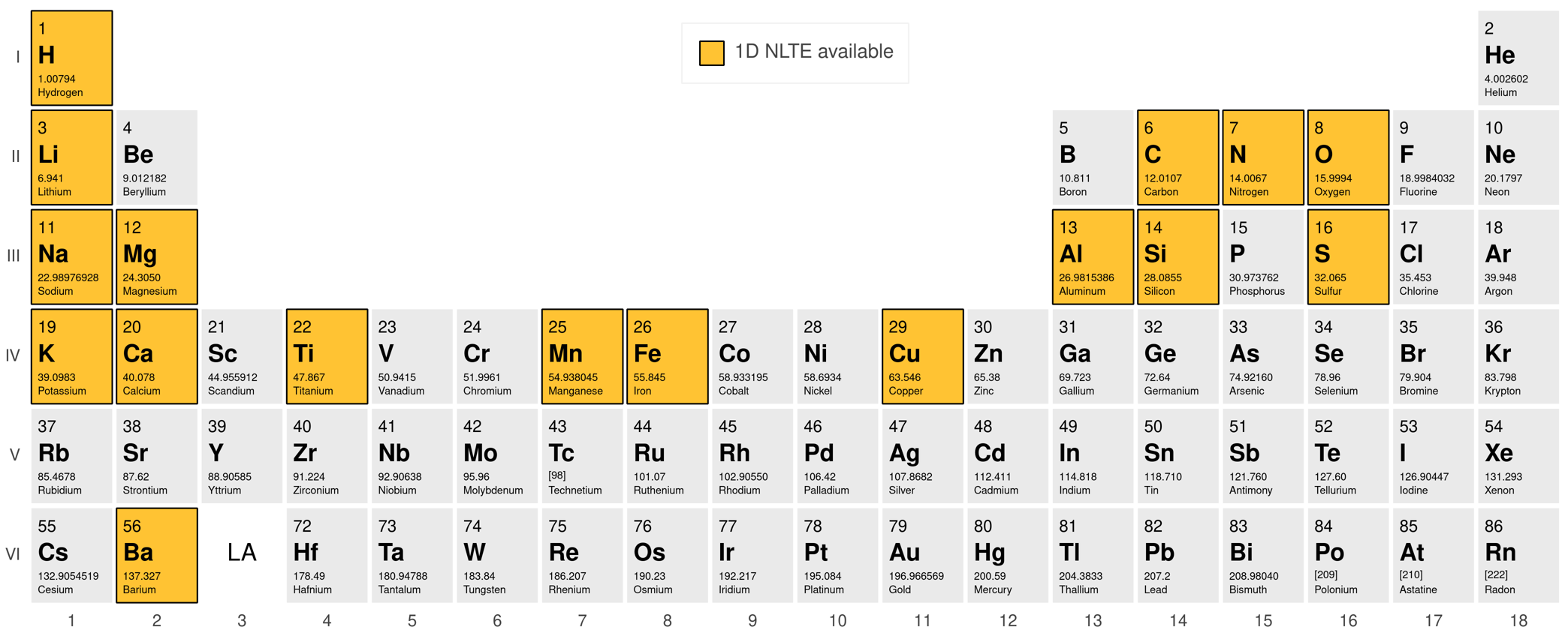
Fig 1: Periodic table highlighting the chemical elements for which 1D NLTE departure coefficients are available in PySME.

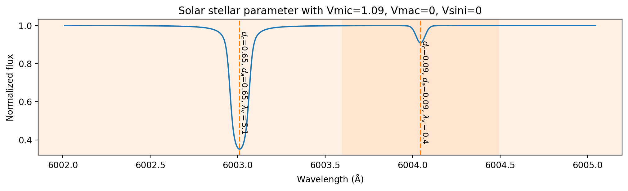
Fig 2: Synthetic spectrum of the example

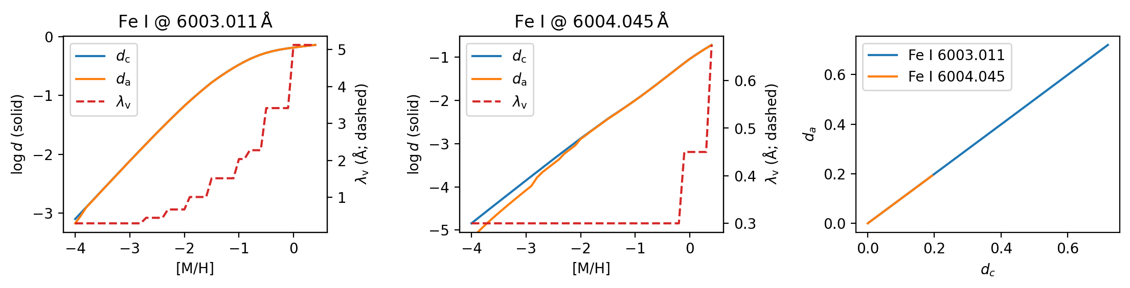
Fig 3: Left and middle panels: growth of dc, da and λv for two example Fe lines with metallicity in solar parameters. Right panel: dc vs da for the

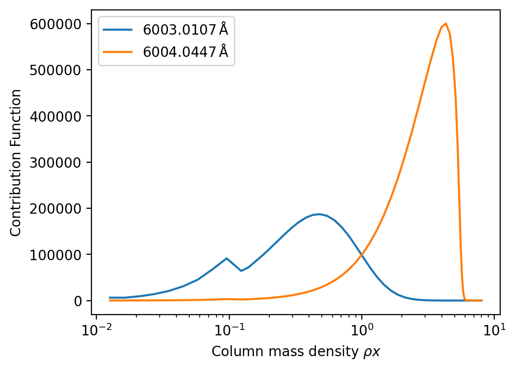
Fig 4: Flux contribution function for the stronger (6003.011 Å) and

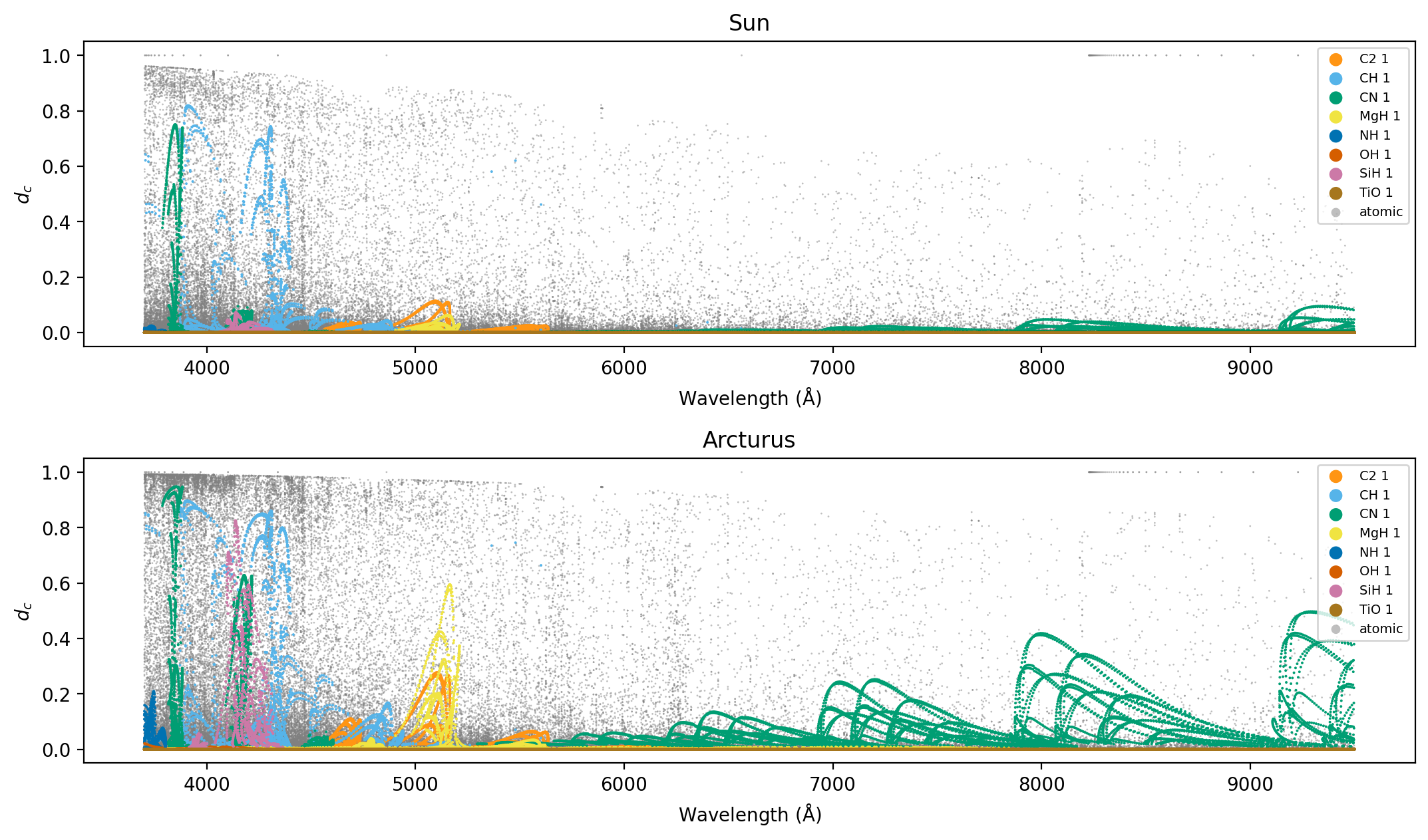
Fig 5: Central depths of optical spectral lines for the Sun (top) and Arcturus (bottom). Coloured points mark molecular features, and grey points

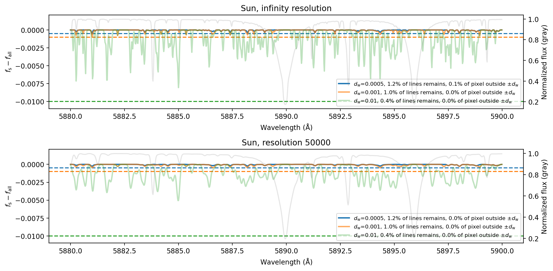
Fig 6: Difference between synthetic spectra computed with negligible lines removed ( fs) and those including all lines ( fall), shown for solar

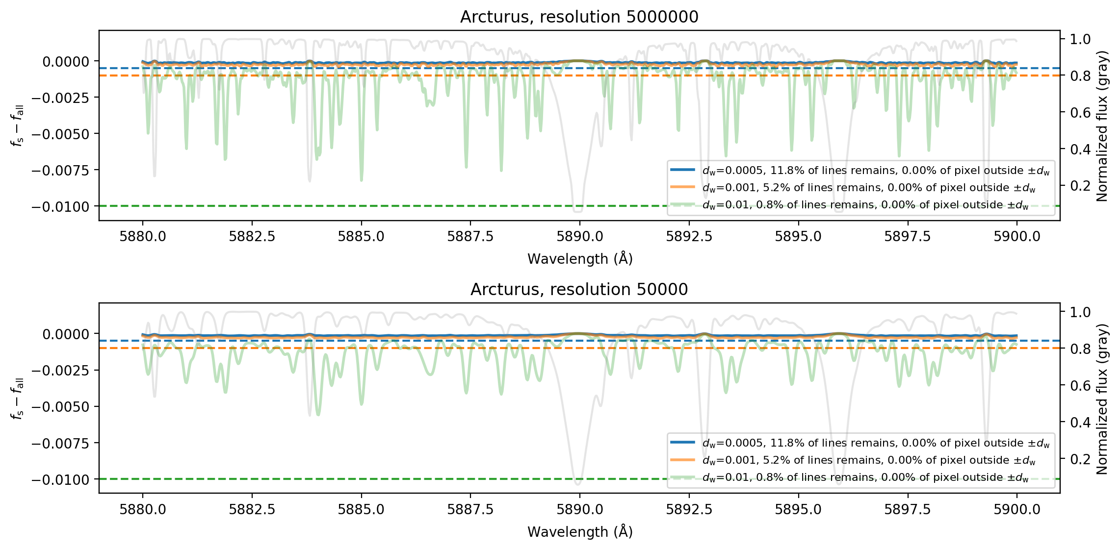
Fig 7: Same as Figure 6, but for the stellar parameters of Arcturus.

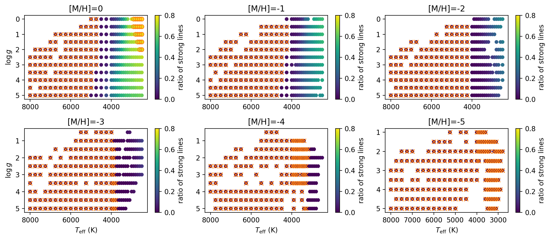
Fig 8: The ratio of non-negligible lines across the Kiel diagram for MARCS grid points. Grid points marked with orange circles indicate locations

Limitations

• The excerpt does not report explicit runtime numbers or speedup factors for the dynamic line-list workflow, only that it improves scalability.
• The validation is mostly deterministic and hand-picked: two stars (Sun and Arcturus), selected Fe I lines, and a TiO-rich spectral region; broader blind testing on diverse stars is not shown in the excerpt.
• The accumulated filtering bin width is fixed at 0.2 Å by default, but the paper does not provide a systematic sensitivity analysis showing how results vary with this choice.
• The database reuse of line diagnostics is conservative, but the excerpt does not quantify how often interpolation/reuse versus recomputation is triggered in realistic survey pipelines.
• NLTE grids are only valid within the tabulated MARCS-based parameter and abundance ranges; extrapolation behavior is not described.
• Uncertainty propagation for derived parameters is flagged as potentially biased, but the paper does not propose a correction method.

Open questions / follow-ons

• How much wall-clock and memory savings does dynamic line-list construction deliver at different line-list sizes and stellar regimes, especially for repeated optimization loops?
• How sensitive is the accumulated negligible-line filtering to the 0.2 Å bin width, the depth threshold dw, and the chosen resolution or broadening kernel?
• Can the conservative database reuse strategy be extended to safer interpolation or uncertainty-aware reuse of line diagnostics across sparse stellar-parameter grids?
• How should uncertainty estimates be adjusted when derived parameters materially influence the spectrum during χ2 minimization?

Why it matters for bot defense

For bot-defense engineers, the direct analogy is not CAPTCHA itself but systems that must balance fidelity against throughput under large candidate sets. The paper is a good example of moving expensive precomputation out of the critical path, caching intermediate diagnostics, and pruning only after defining a conservative local grouping rule. That design pattern applies to high-volume risk scoring, feature extraction, and any pipeline where naive per-item filtering can miss clustered weak signals that matter in aggregate.

The most transferable idea is the combination of a human-interpretable threshold with a conservative accumulation rule. In bot detection, that maps well to grouped signals such as short-session bursts, linked device fingerprints, or clusters of weak anomalies that individually look benign. The paper also reinforces a practical caution: when you introduce derived quantities or cached intermediate state, you can improve performance, but you must track when those approximations distort downstream uncertainty or cause stale decisions under distribution shift.

Cite

@article{arxiv2605_04007,
  title={ PySME v1.0: improved modelling of stellar spectra for survey-scale applications },
  author={ Mingjie Jian and Nikolai Piskunov and Jeff Valenti and Ella Xi Wang and Brian Thorsbro and Henrik Jönsson and Ansgar Wehrhahn },
  journal={arXiv preprint arXiv:2605.04007},
  year={ 2026 },
  url={https://arxiv.org/abs/2605.04007}
}

Read the full paper

• arXiv:2605.04007 (abstract)
• arXiv:2605.04007 (PDF)