Precomputed Lens Transport Maps

Source: arXiv:2605.04017 · Published 2026-05-05 · By Yang Chen, Xiaochun Tong, Afet Abzar, Leo Hanxu, Matthew Avolio, Toshiya Hachisuka

TL;DR

This paper addresses a practical gap in camera/lens simulation: existing fast approximations either model only geometry (pinhole, thin lens, ABCD, polynomial optics) or only the smooth refraction component, but they do not jointly capture wavelength dependence, occlusion/discontinuities from apertures and housing, and Fresnel throughput needed for lens flares. The authors propose a precomputed lens transport map that learns path-specific ray mappings with a factorized classifier-regressor design: a classifier rejects invalid/occluded rays, and a regressor predicts output ray position, direction, and Fresnel intensity for valid rays. A further design choice is to use tanh MLPs, motivated by the claim that the physically valid path map is at least C1 within each valid region.

The main result is that the learned model matches ray tracing more closely than Taylor polynomial optics, especially for longer and more off-axis paths where polynomial truncation and accumulation error become visible. The system also supports both forward lens flare rendering and backward path tracing for depth of field, while being substantially faster than brute-force ray tracing (the abstract states “an order of magnitude faster”; one reported example in Fig. 1 shows 74.4 s for Ours vs 1180.3 s for RT at 32768 spp for a 24 mm lens scene). The paper’s emphasis is not just speed, but unifying multiple lens effects in one precomputed representation instead of maintaining separate approximations for flare, DOF, and chromatic aberration.

Key findings

• The model explicitly predicts Fresnel throughput, which prior polynomial and neural ray-mapping approaches omitted; this is presented as necessary for accurate lens flare brightness and internal reflection effects.
• The classifier-regressor factorization improves handling of discontinuities from aperture/barrel occlusion by filtering invalid rays before regression; Fig. 7 shows the no-classifier variant produces an overly exposed incorrect image.
• The method is wavelength-aware and is designed to capture chromatic aberration without per-wavelength polynomial fits; the paper contrasts this with prior polynomial models that approximate each wavelength separately.
• For lens flare rendering, Fig. 8 reports better visual agreement than Taylor polynomial optics, especially for longer paths and wider-FOV lenses (the paper specifically notes the 22 mm lens is harder for the polynomial baseline).
• For depth-of-field rendering, Fig. 9 reports mean absolute percentage error (MAPE) values all below 0.15 and often below 0.05 across two scenes and three lens designs.
• The implementation uses approximately 81 million valid samples per path type for regressor training, occupying about 4.27 GB per path; classifier data uses a balanced valid/invalid set of about 1.85 GB per path.
• Training is done with compact 32-neuron tanh MLPs; the regressor uses 5 hidden layers and the classifier uses 2 hidden layers, with lr=1e-4 decayed by 0.95 every 10,000 batches.
• Fig. 1’s runtime example reports 74.4 s for Ours vs 1180.3 s for ray tracing at 32768 spp for one lens-flare scene, which is roughly 15.9× faster in that case.

Methodology — deep read

Threat model and assumptions: this is not a security paper, so the “threat” is computational and physical-model mismatch rather than an adversary. The method assumes a static lens system with rotational symmetry about a common optical axis and geometric optics (no wave optics). It further assumes that a ray path can be decomposed into a finite sequence of interactions (reflections/transmissions) and that each path type can be modeled independently. The key practical assumption is that most useful contributions come from short paths; the authors state that under typical absorption assumptions, higher-order paths with more than two bounces contribute negligibly, so they focus on those paths.

Data generation and labels: training data are produced by a custom ray-tracing simulator that ingests lens configurations from JSON exported by Open Optical Designer. For each path type, the authors uniformly sample input position and direction within the valid region, and importance-sample wavelength according to the CIE XYZ color matching function. Because the valid set is sparse, they use MCMC with a binary visibility target function to efficiently generate samples. The regressor dataset contains approximately 81 million valid samples per path type, about 4.27 GB of storage. The classifier dataset is balanced with equal valid and invalid rays, requiring about 1.85 GB per path. The paper does not state a held-out split ratio in the excerpt, nor whether splits are by lens, by path, or purely random within a path; that matters because random splits could overestimate generalization if neighboring samples are highly correlated.

Architecture and algorithm: the method decomposes the global transport map T into path-specific maps T^P, where P is a sequence of reflection/transmission events. This is conceptually important because the mapping is multi-valued: a single incident ray may produce zero, one, or many outputs depending on occlusion and Fresnel splitting. Each path type gets its own small MLP pair: a classifier g(x) predicts whether an input belongs to the valid domain Ω_P for that path, and a regressor f(x) predicts the output ray state only when g(x)=1. The regressor outputs output position, output direction, and intensity/Fresnel throughput. The authors use tanh activations in hidden layers and no output activation. The regressor is a 5-hidden-layer MLP with 32 neurons per layer and losses of MSE for position/intensity plus cosine similarity for direction; the classifier is a 2-hidden-layer MLP trained with binary cross-entropy. The motivation for tanh is that, after occluded regions are removed, the underlying map should be smooth (at least C1) within the valid region, whereas ReLU’s piecewise linear kinks can cause striping artifacts in rendered images.

Training regime and one concrete pipeline example: training uses Adam-like optimization details only partially specified in the excerpt; the paper states an initial learning rate of 1e-4 that decays exponentially by 0.95 every 10,000 batches. The light-tracing regressors are trained for 40 epochs with batch size 8192. For the full-transmittance regressor used in backward path tracing, training is done in two phases: 200 epochs with batch size 32768, then 50 epochs of fine-tuning with batch size 8192 and a reduced starting learning rate of 1e-6. Inference is integrated into LuisaRender by fusing the MLP into GPU compute kernels and approximating tanh with a rational function. A concrete forward-light-tracing example is: sample an input ray on the forward input plane, use the classifier to reject rays blocked by the barrel/aperture, pass valid rays to the regressor to get (p_out, w_out, I_out), then splat the contribution into the sensor image with the dot product between w_out and the sensor normal as the geometric factor. For backward path tracing, the same classifier-regressor pair maps sensor-adjacent samples back through the lens to scene rays; only fully transmitted paths are used for the camera integrator.

Evaluation protocol and reproducibility: the paper evaluates against Taylor polynomial optics [Hullin et al. 2012] and brute-force ray tracing, using both qualitative figures and quantitative error for depth-of-field. For lens flares, the paper traces one million rays per RGB channel and explicitly disables Fresnel throughput in the polynomial baseline because that baseline does not support it. Fig. 8 is used to show that polynomial error grows for longer paths and wider FOV lenses, while the learned method remains closer to ray tracing. Fig. 7 isolates the classifier’s effect by comparing renders with and without the classifier; without it, invalid rays hit the aperture/barrel and brighten the image incorrectly. Fig. 4 compares ReLU and tanh MLPs and shows striping artifacts for ReLU. Reproducibility is partial: the paper specifies the source of lens configurations (Open Optical Designer JSON) and the integration framework (LuisaRender), but the excerpt does not mention public code, frozen weights, or a released dataset. If those are absent, reproducing the exact training set would require re-running the ray tracer and MCMC sampler.

Technical innovations

• A path-factorized lens transport model that predicts valid/invalid ray outcomes separately from the smooth geometric regression, avoiding domain subdivision used by prior neural lens models.
• Explicit Fresnel throughput prediction inside the learned transport map, enabling lens flare simulation rather than only refraction-only image formation.
• Wavelength-aware neural transport without per-wavelength polynomial fitting, letting a single model represent chromatic effects.
• A tanh-based MLP design justified by the claim that the valid transport map is C1 within each path domain, reducing striping artifacts seen with ReLU.

Datasets

• Per-path regressor dataset — ~81 million valid samples per path type — generated by custom ray tracing from Open Optical Designer lens JSONs
• Per-path classifier dataset — balanced valid/invalid rays, about 1.85 GB per path — generated by custom ray tracing from Open Optical Designer lens JSONs

Baselines vs proposed

• Taylor polynomial optics [Hullin et al. 2012]: qualitative lens flare rendering is less accurate than proposed, especially for longer paths and the 22 mm lens in Fig. 8; no single scalar metric reported in the excerpt.
• Ray tracing (reference): Fig. 1 reports 74.4 s for proposed vs 1180.3 s for RT at 32768 spp on the shown 24 mm lens scene (about 15.9× faster); the paper also says “an order of magnitude faster” in the abstract.
• ReLU MLP vs tanh MLP: Fig. 4 qualitatively shows ReLU produces strip-like artifacts while tanh yields smoother patterns; no numeric metric reported.
• Without classifier vs with classifier: Fig. 7 qualitatively shows the no-classifier variant produces an overly exposed, incorrect render; no numeric metric reported.

Figures from the paper

Figures are reproduced from the source paper for academic discussion. Original copyright: the paper authors. See arXiv:2605.04017.

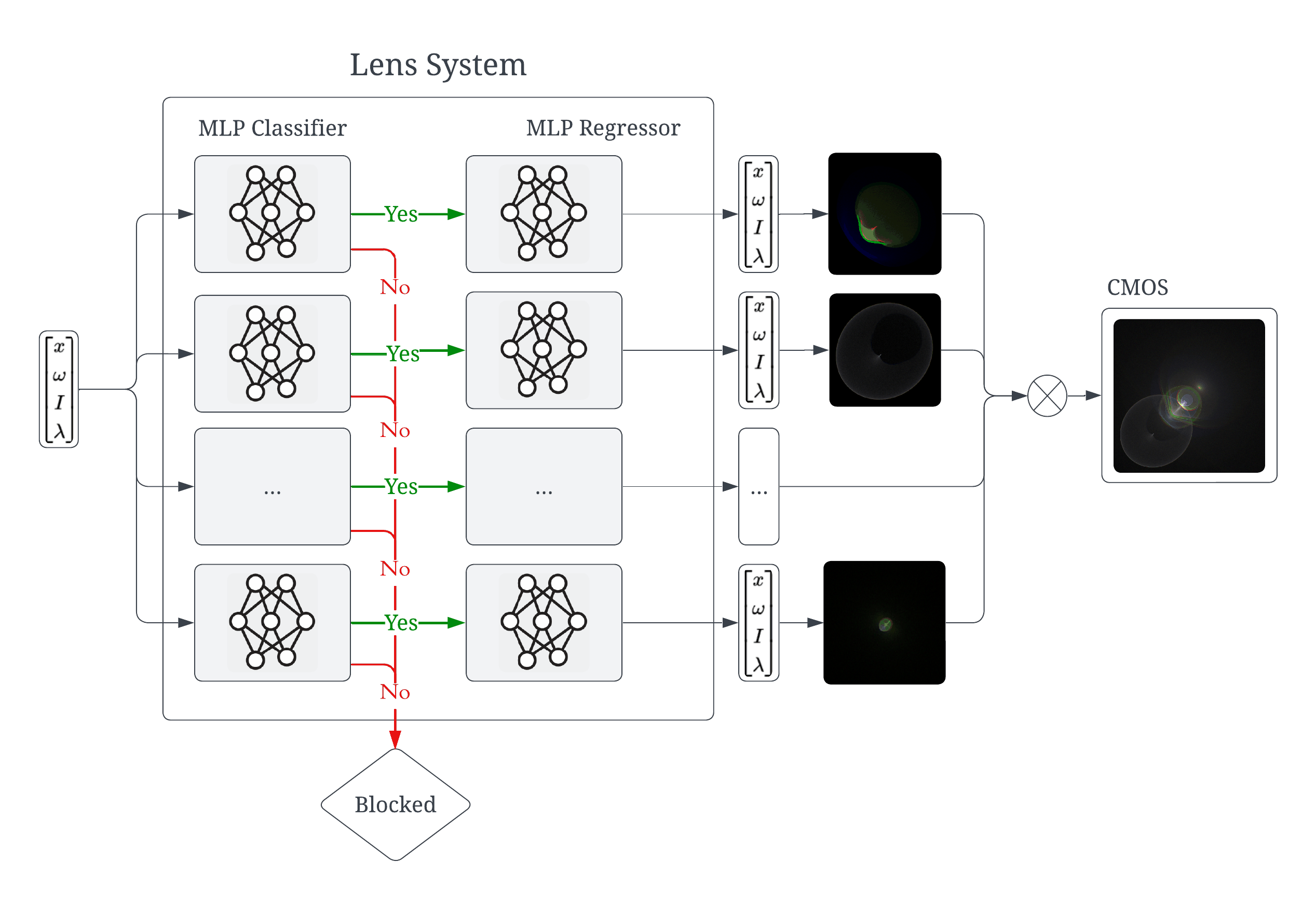
Fig 1: Left: Overview of our forward pass pipeline for lens flare rendering. Middle: Comparison of lens flare results between ray tracing (RT) and our neural

Fig 2: We decompose light transport paths in a lens system into many

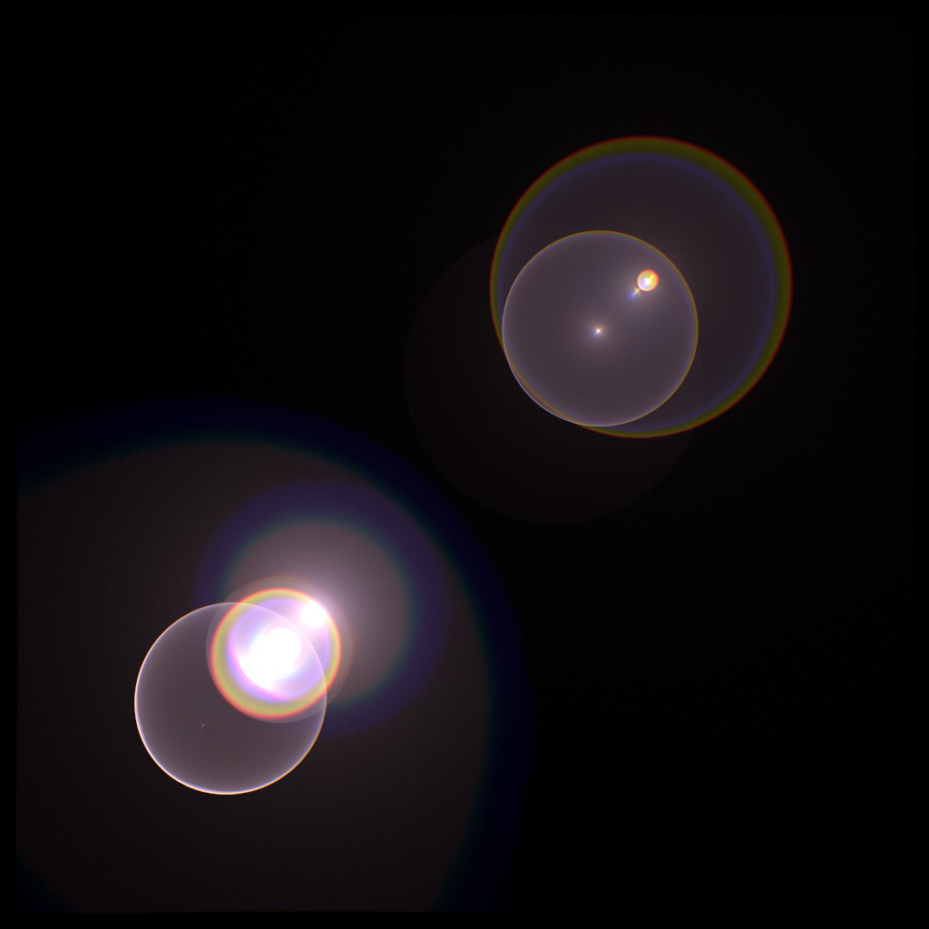
Fig 3 (page 1).

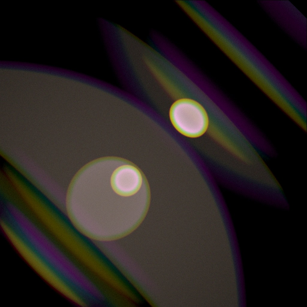
Fig 4 (page 1).

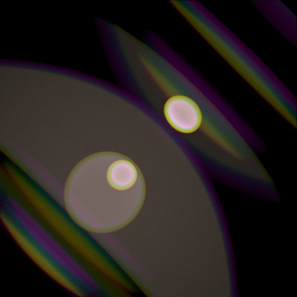
Fig 5 (page 1).

Fig 6 (page 1).

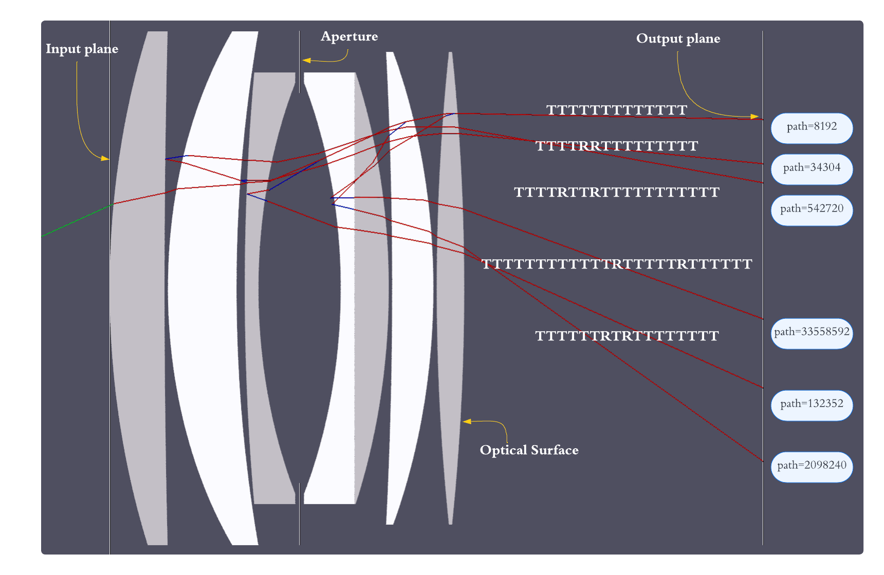
Fig 3: We plot the intensity for two type of path in the 3D input space. For

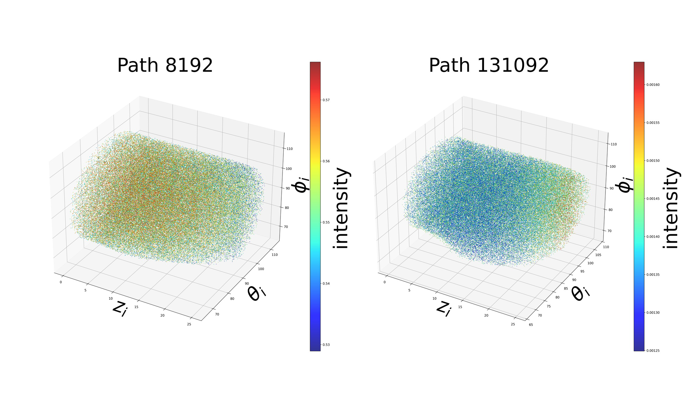
Fig 4: We compared the lens flares produced by a ReLU MLP and tanh

Limitations

• The method assumes static, rotationally symmetric lens systems under geometric optics; it does not target dynamic lens assemblies, decentering, or wave-optical effects.
• The excerpt does not specify a public code release, released dataset, or frozen weights, so external reproducibility may be limited.
• Evaluation appears focused on a small set of lens designs shown in figures; generalization across a broader optical catalog is not established in the excerpt.
• The paper notes higher-order paths (>2 bounces) are negligible under typical absorption assumptions, but does not deeply validate that assumption across all lens types or flare-heavy scenes.
• The full-transmittance model is only used for fully transmitted paths in backward path tracing; reflected paths for camera rendering are not modeled in that integrator.
• Quantitative results in the excerpt are limited; many comparisons are visual rather than reported as standardized error metrics.

Open questions / follow-ons

• Can the factorized classifier-regressor design be extended to non-rotationally symmetric lenses or misaligned optics without exploding the number of path-specific models?
• How many path types are actually necessary in flare-heavy or highly reflective lenses before higher-order interactions become non-negligible in the final image?
• Would a single shared backbone with path-conditioned heads outperform the current per-path small MLPs in memory, training time, or cross-lens transfer?
• Can the learned transport map be differentiated reliably enough for lens design optimization, as hinted by the authors, without introducing gradient artifacts at path boundaries?

Why it matters for bot defense

For bot-defense and CAPTCHA practitioners, this paper is relevant mainly as a modeling pattern: separate discrete validity/occlusion decisions from continuous regression. In CAPTCHA or anti-bot pipelines, many signals have the same structure as lens transport here: a sparse valid region with sharp discontinuities, plus a smooth field inside that region. The classifier-regressor factorization is a reminder that forcing one regressor to learn both “is this input meaningful?” and “what is the value?” often hurts accuracy near boundaries.

A second takeaway is the activation-function choice. The authors argue that once you isolate the valid manifold, a C1-smooth regressor can reduce visual artifacts compared with ReLU. In bot-defense systems, that translates to preferring smooth calibrated scoring models when the downstream decision boundary is expected to be physically or semantically smooth, while using a separate gate to handle hard invalid/blocked cases. The caveat is that this is a lens-simulation paper, not an adversarial security study, so the transfer is methodological rather than directly operational.

Cite

@article{arxiv2605_04017,
  title={ Precomputed Lens Transport Maps },
  author={ Yang Chen and Xiaochun Tong and Afet Abzar and Leo Hanxu and Matthew Avolio and Toshiya Hachisuka },
  journal={arXiv preprint arXiv:2605.04017},
  year={ 2026 },
  url={https://arxiv.org/abs/2605.04017}
}

Read the full paper

• arXiv:2605.04017 (abstract)
• arXiv:2605.04017 (PDF)