Flow Sampling: Learning to Sample from Unnormalized Densities via Denoising Conditional Processes

Source: arXiv:2605.03984 · Published 2026-05-05 · By Aaron Havens, Brian Karrer, Neta Shaul

TL;DR

Flow Sampling is a diffusion-style sampler for unnormalized target densities when you can evaluate the energy or reward gradient but you do not have target samples. The core problem is amortizing expensive sampling from a known-but-unnormalized distribution q(x) ∝ exp(r(x)) / Z, where MCMC is too slow and many prior diffusion samplers still rely on repeated target evaluations, Monte Carlo correction, or auxiliary networks. The authors flip the usual flow-matching setup: instead of conditioning on data samples and learning a noising process, they condition on source samples and learn a denoising conditional process whose regression target can be written in closed form from endpoint score information.

What is new is a replay-buffer training scheme built around a conditional drift formula that reuses a single energy-gradient evaluation per target sample along an entire interpolant trajectory. In the Euclidean case they derive a closed-form target drift for a linear interpolant; on constant-curvature manifolds they further derive a closed-form geodesic conditional drift, including hyperspheres and hyperbolic spaces. Empirically, the paper reports strong results on synthetic Lennard–Jones and double-well benchmarks, peptide conformers, and spherical mixtures, with lower training compute than prior adjoint-based and Monte Carlo-corrected diffusion samplers while matching or improving sample quality.

Key findings

• On synthetic energy benchmarks, Flow Sampling achieves the best reported E(·)W2 on all three tasks in Table 1: DW-4 0.11±0.04, LJ-13 0.97±0.53, and LJ-55 21.32±0.63.
• On DW-4, Flow Sampling improves geometric W2 from 0.43±0.05 for ASBS to 0.36±0.03 and E(·)W2 from 0.20±0.11 to 0.11±0.04 (Table 1).
• On LJ-13, Flow Sampling reduces E(·)W2 from 1.99±1.01 (ASBS) to 0.97±0.53 and slightly improves geometric W2 from 1.59±0.03 to 1.58±0.01 (Table 1).
• On LJ-55, Flow Sampling lowers E(·)W2 from 28.10±8.15 (ASBS) to 21.32±0.63 and geometric W2 from 4.00±0.03 to 3.98±0.01 (Table 1).
• In Ala2, Flow Sampling at NFE(train)=1024 reaches DKL 0.031±0.004 on ϕ and 0.008±0.002 on ψ, compared with ASBS at 1024 of 0.504±0.006 and 0.726±0.300, respectively (Table 2).
• In Ala2, the joint torsion JSD drops from 0.242±0.042 for ASBS at 1024 to 0.018±0.001 for Flow Sampling at 1024, while energy W2 drops from 8.650±0.371 to 0.637±0.267 (Table 2).
• On SPICE conformer generation, Flow Sampling at NFE(train)=256 attains recall 91.89±7.51 and AMR 0.86±0.23 on the held-out SPICE test set, compared with ASBS at 512 NFE/train with recall 89.66±19.42 and AMR 0.86±0.24 (Table 3).
• The paper states Flow Sampling reduces simulation/training cost by 4–8× on large-scale amortized molecular conformer generation, but the exact compute accounting is discussed qualitatively in Section 6.5 rather than as a single end-to-end wall-clock number.

Threat model

The adversary is not a malicious attacker but the difficulty posed by expensive unnormalized target evaluation. The method assumes access to an evaluable reward/energy r(x) and its gradient ∇r(x), plus an easy-to-sample source p0 such as a Gaussian; it does not assume target samples from q. It also assumes the sampler can draw from its own current model with Euler–Maruyama and can store endpoint-score pairs in a replay buffer. What it cannot do is rely on exact normalization constants or cheap direct samples from q; for the manifold case it additionally assumes constant curvature so that geodesics, parallel transport, and Jacobians are closed form.

Methodology — deep read

The threat model is not a security attacker model in the CAPTCHA sense; it is a sampling-computation setting. The user is assumed to know the unnormalized target up to a scalar-normalization constant: they can evaluate r(x) and its gradient ∇r(x), but cannot draw i.i.d. samples from q. The sampler must work in high dimensions, sometimes on curved manifolds, and should minimize expensive energy/score evaluations. The authors explicitly position the method against MCMC, Langevin, diffusion samplers with Monte Carlo corrections, and adjoint/Schrödinger-bridge-style methods that need auxiliary components or repeated target queries.

Data provenance depends on the benchmark. For synthetic experiments, the targets are known n-particle energy systems: DW-4 in 2D, LJ-13 in 3D, and LJ-55 in 3D; the paper compares against long-run MCMC reference samples and evaluates geometric W2 plus an energy-histogram W2 (Table 1). For peptides, the targets are classical force-field distributions for Ala2 (22 atoms) and Ala4 (42 atoms) with implicit water via OpenMM; ground truth comes from long MD simulation, and evaluation uses torsion-angle KL/JSD and energy W2 (Table 2). For amortized conformer generation, the paper trains on 24,775 SPICE molecular topologies and evaluates on 80 held-out SPICE molecules plus 80 GEOM-DRUGS molecules, following the protocol of Havens et al. (2025) (Table 3). For the manifold experiment, the target is a synthetic mixture of von Mises–Fisher components on S2; the paper does not specify the exact K in the excerpt, only that the means lie on coordinate axes and diagonal directions.

Architecturally, Flow Sampling starts from the flow-matching identity that a deterministic transport path can be turned into a diffusion with the same marginals by adding a score term to the drift (Proposition 3.1). The key inversion is to condition on source samples X0 ~ p0 rather than target samples X1 ~ q. They define a conditional path pt|0 as a pushforward of the target distribution, pt|0(x|x0) = αt^{-d} q((x - σt x0)/αt), and identify a conditional velocity vt|0(x|x0) = (dot αt/αt)(x - σt x0) + dot σt x0. The supervising diffusion drift is then ut|0 = vt|0 + (g_t^2/2)∇log pt|0, which at the interpolant Xt = σt X0 + αt X1 becomes a closed-form expression involving only X1, X0, and the target score ∇r(X1): ut|0(Xt|x0) = dot αt X1 + dot σt x0 + (g_t^2/(2αt))∇r(X1) (Proposition 3.2). They use the linear schedule αt=t, σt=1−t, g_t^2=2γt, which makes the target scale as X1 − X0 + γ∇r(X1). The model itself is a drift network u_θ(x,t) trained by mean-squared error against this target drift.

Training is two-phase and replay-buffer based. In the exploration phase, the current detached model u_{\bar θ} is rolled forward with Euler–Maruyama from X0 ~ N(0,I) to produce X\barθ_1; the energy gradient ∇r(X\barθ_1) is evaluated once and stored. In the optimization phase, batches are drawn from the buffer, a fresh X0 and t are sampled, the interpolant Xt=(1−t)X0+tX\barθ_1 is formed, and the target drift is X\barθ_1 − X0 + γ∇r(X\barθ_1). The model is updated with MSE loss to regress onto this target. The important efficiency claim is that the expensive gradient of the reward/energy is evaluated only at sampled endpoints from the current detached model, not at every intermediate time point along the path.

For manifold extension, the paper replaces Euclidean interpolation with geodesic interpolation on a constant-curvature manifold M embedded in an ambient space A = R^{d+1}. The diffusion is projected to the tangent space using P^⊥x, and the solver uses the exponential map exp_x with projected Brownian increments. The conditional path is the geodesic ϕ_t(X1|x0)=exp[(1−t)log_{X1}(x0)], and the conditional score decomposes into a transported target gradient term plus a Jacobian-determinant correction. Proposition 4.1 gives a closed-form Jacobian J_t expressed through parallel transport and a scalar curvature-dependent factor c_t, with explicit formulas for the hypersphere case: SLERP for the geodesic, Householder reflection for parallel transport, and a closed-form ∇_M log det(J_t). The Riemannian loss projects the predicted drift to the tangent space and regresses it to the closed-form conditional drift.

Evaluation uses task-appropriate metrics and baselines. On synthetic systems, the main metrics are geometric W2 and energy-histogram W2 relative to long-run MCMC ground truth; baselines are PIS, DDS, iDEM, AS, and ASBS, all using a 5-layer EGNN, while Flow Sampling XL uses 10 layers. On Ala2, they report 1D marginal DKLs for ϕ and ψ, 2D JSD for the joint torsion distribution, and energy W2; they also compare degradation as training NFE drops from 1024 to 64. On Ala4, they present a qualitative mode-coverage study over three torsions showing 2^3=8 metastable modes. On SPICE/GEOM-DRUGS, they report coverage recall, precision, and AMR at a 1.25 Å threshold, with a 12-layer EGNN across methods; they note precision coverage was not reported for ASBS. The paper reports mean and standard error across 5 training runs in Table 1, but the excerpt does not describe any formal statistical tests, cross-validation, or confidence-interval testing beyond those repeated runs.

Reproducibility is partial from the excerpt. The authors provide algorithmic pseudocode (Algorithm 1) and specify core schedules (linear αt, σt, g_t^2), model families (EGNN, PaiNN), and benchmark protocols. They also cite a replay-buffer implementation and a manifold solver. However, the excerpt does not mention code release, exact hyperparameters such as learning rates or batch sizes, random seed strategy, optimizer details beyond generic gradient descent, or whether frozen weights/datasets are publicly released. One concrete end-to-end example from the paper is Ala2: a full-atom peptide force-field target is trained with the same E(3)-equivariant PaiNN as ASBS; Flow Sampling at 1024 training NFE uses detached samples from its own current model, evaluates the classical force-field gradient once per stored endpoint, and then regresses the network on linear interpolants to match the target drift; it then evaluates sample quality against MD-generated torsional ground truth using DKL, JSD, and energy W2.

Technical innovations

• A conditional denoising diffusion objective for unnormalized densities that conditions on source noise samples rather than target data samples, enabling data-free sampler learning.
• A closed-form drift target for linear interpolants that reuses a single endpoint score evaluation ∇r(X1) across all t, reducing energy-evaluation cost via a replay buffer.
• A Riemannian extension of flow sampling on constant-curvature manifolds with closed-form conditional drift terms using geodesic interpolation, parallel transport, and Jacobian corrections.
• A practical fixed-point / detached-policy training loop that alternates exploration and optimization, similar in spirit to replay-buffer off-policy learning but specialized to energy-based sampling.

Datasets

• DW-4 — synthetic n-particle benchmark, N=4, d=2 — generated from the double-well potential
• LJ-13 — synthetic n-particle benchmark, N=13, d=3 — generated from the Lennard-Jones potential
• LJ-55 — synthetic n-particle benchmark, N=55, d=3 — generated from the Lennard-Jones potential
• Ala2 — 22 atoms — classical force-field with implicit water via OpenMM
• Ala4 — 42 atoms — classical force-field with implicit water via OpenMM
• SPICE — 24,775 molecular topologies for training; 80 held-out molecules for test — public SPICE dataset
• GEOM-DRUGS — 80 molecules for generalization evaluation — public GEOM-DRUGS dataset
• S2 vMF mixtures — synthetic spherical benchmark — constructed mixture on the unit sphere

Baselines vs proposed

• PIS: DW-4 geometric W2 = 0.68±0.23 vs proposed: 0.36±0.03
• DDS: DW-4 geometric W2 = 0.92±0.11 vs proposed: 0.36±0.03
• iDEM: DW-4 energy W2 = 0.55±0.14 vs proposed: 0.11±0.04
• AS: LJ-13 energy W2 = 2.40±1.25 vs proposed: 0.97±0.53
• ASBS: LJ-55 energy W2 = 28.10±8.15 vs proposed: 21.32±0.63
• ASBS: Ala2 joint JSD = 0.242±0.042 vs proposed: 0.018±0.001
• ASBS: SPICE recall = 89.66±19.42 vs proposed: 91.89±7.51
• RDKit ETKDG: SPICE coverage recall = 72.74±33.18 vs proposed: 91.89±7.51

Figures from the paper

Figures are reproduced from the source paper for academic discussion. Original copyright: the paper authors. See arXiv:2605.03984.

Fig 1: Flow Sampling is the first diffusion sampler able to perform sampling from an unnormalized density on Riemannian manifolds.

Fig 2: (left) Flow matching conditional probability path is marginal of a noising process conditioned on a data point x1. (middle) Flow

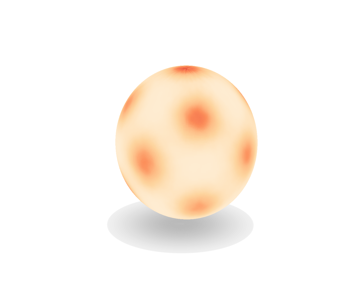
Fig 3 (page 2).

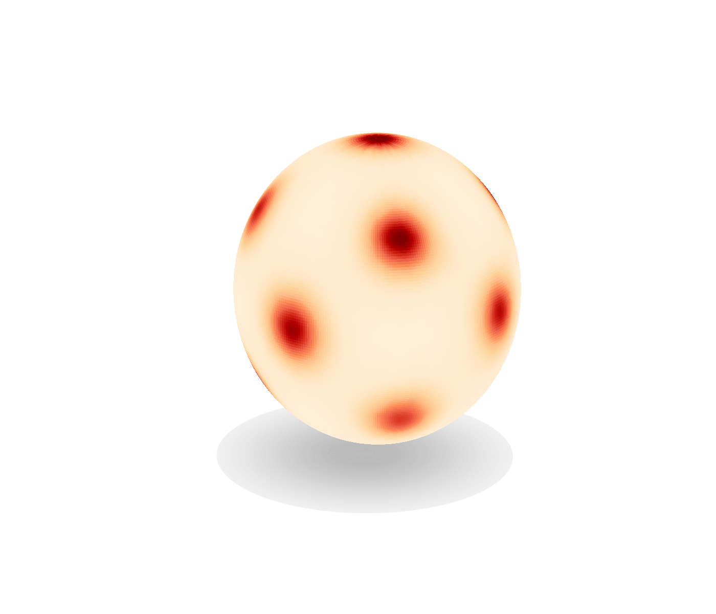
Fig 4 (page 2).

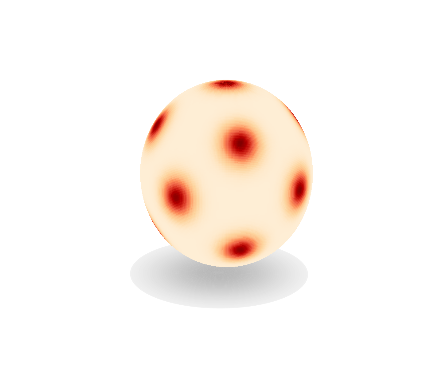
Fig 5 (page 2).

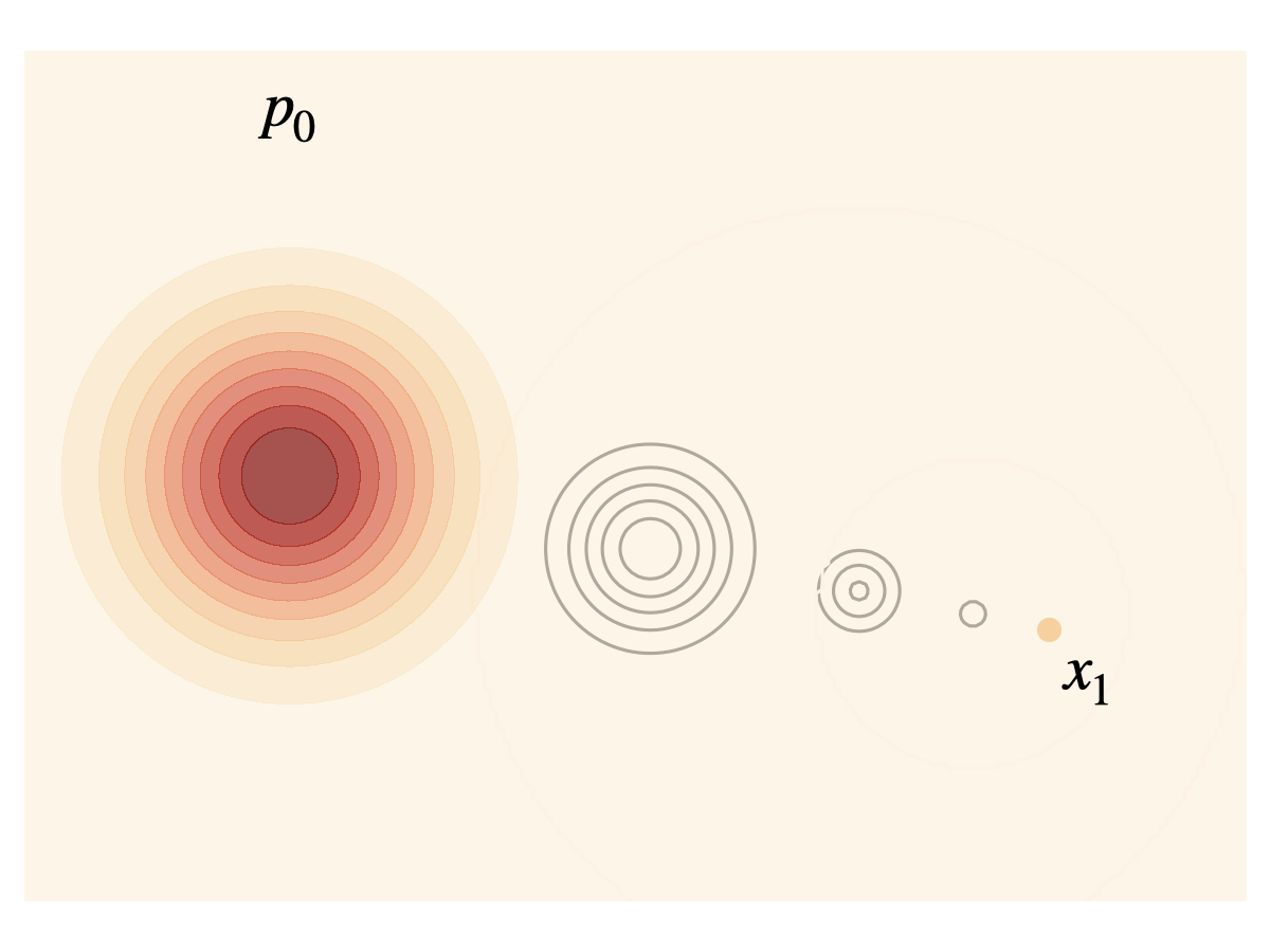
Fig 6 (page 3).

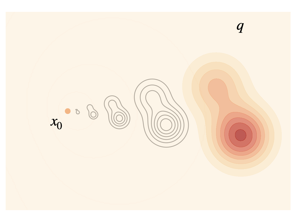
Fig 7 (page 3).

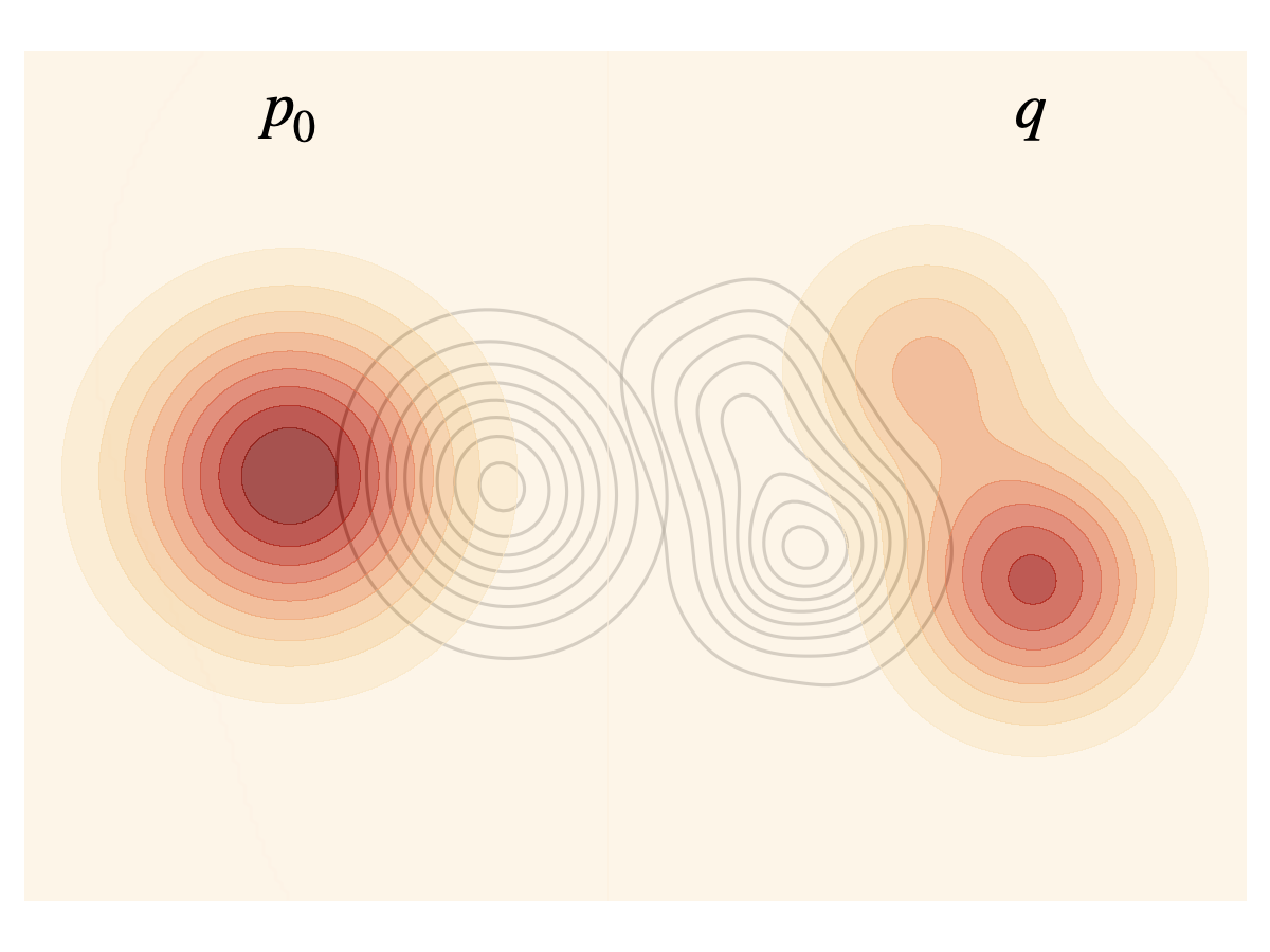
Fig 8 (page 3).

Limitations

• The paper’s strongest claims are empirical, but several experimental details are only partially visible in the excerpt, including exact optimizer settings, batch sizes, learning-rate schedules, and random seeds.
• The core efficiency claim hinges on reduced energy-gradient evaluations and lower NFE during training, but the excerpt mostly reports relative counts rather than unified wall-clock, FLOP, or dollar-cost measurements.
• The Riemannian extension is derived for constant-curvature manifolds, so it does not directly cover arbitrary manifolds or settings where closed-form exponential/log maps are unavailable.
• Some comparisons are not perfectly symmetric: ASBS uses an auxiliary network and a pretraining step in some contexts, while the Flow Sampling comparisons sometimes omit those extras or use reimplementation variants.
• For the manifold and synthetic benchmarks, the targets are well-defined and controlled; it remains unclear how the method behaves on noisier scientific objectives with approximate gradients or expensive stochastic energy estimators.
• The excerpt does not specify whether code, checkpoints, or exact benchmark configurations are publicly released, which limits reproducibility assessment.

Open questions / follow-ons

• Can the replay-buffer conditional-drift trick be extended to targets with only approximate or stochastic gradients, such as noisy free-energy estimators?
• How sensitive is Flow Sampling to the choice of γ, the exploration/optimization schedule, and the quality/diversity of replay-buffer endpoints?
• Can the manifold derivation be generalized beyond constant curvature to practical geometries used in robotics, chemistry, or constrained optimization?
• Would combining Flow Sampling with a lightweight correction mechanism recover exactness or improve tail coverage without reintroducing the high evaluation cost of prior methods?

Why it matters for bot defense

For bot-defense, the main takeaway is methodological rather than directly deployable: the paper shows how to learn an amortized sampler when you can score a target but cannot sample from it. That is conceptually adjacent to CAPTCHA/bot-defense settings where you may have a reward or anomaly score over candidate behaviors, challenge parameters, or synthetic adversarial traffic and want to generate diverse high-scoring examples quickly. The replay-buffer and closed-form conditional-drift ideas suggest a way to reduce expensive scoring calls when training generators or simulators for red-teaming and synthetic bot traffic.

A bot-defense engineer should also read this as a warning about adaptive attackers: if the target objective is differentiable and costly but queryable, an attacker may be able to learn a sampler that concentrates on hard cases with much lower online cost than MCMC-style search. The manifold extension is especially relevant if your state space is constrained or directional, such as browser fingerprint manifolds, posture/gesture spaces, or structured policy parameters. Defensively, that means designing challenge spaces and scoring functions that are either non-differentiable, partially hidden, or rate-limited, and evaluating robustness against learned samplers rather than just random search.

Cite

@article{arxiv2605_03984,
  title={ Flow Sampling: Learning to Sample from Unnormalized Densities via Denoising Conditional Processes },
  author={ Aaron Havens and Brian Karrer and Neta Shaul },
  journal={arXiv preprint arXiv:2605.03984},
  year={ 2026 },
  url={https://arxiv.org/abs/2605.03984}
}

Read the full paper

• arXiv:2605.03984 (abstract)
• arXiv:2605.03984 (PDF)