Reconstruction of glymphatic transport fields from subject-specific imaging data, with particular emphasis on cerebrospinal fluid flow and tracer conservation

Source: arXiv:2605.00730 · Published 2026-05-01 · By A. Derya Bakiler, Michael J. Johnson, Michael R. A. Abdelmalik, Frimpong A. Baidoo, Andrew Badachhape, Ananth V. Annapragada et al.

TL;DR

This paper tackles a very specific inverse-problem pain point in image-based transport modeling: if you try to reconstruct flow and clearance fields directly from noisy spatiotemporal imaging, the inferred fields often violate basic physics, especially mass conservation. The authors focus on glymphatic transport in a mouse brain, where contrast-enhanced MRI (CE-MRI) shows tracer movement through CSF pathways. Their central move is to combine an advection-diffusion model with a velocity decomposition that separates a measured/non-solenoidal velocity into a coarse field and a corrective fine-scale field, then solve for the correction so the reconstructed transport is weakly divergence-free.

What is new here is less a new biological hypothesis than a numerical inverse-modeling framework: they adapt the Hughes–Wells conservative advection-diffusion idea from forward stabilization into an inverse setting, and they implement it with immersed isogeometric analysis (IGA) using quadratic B-splines / THB-splines on a nonconforming domain representation. In the reported mouse-brain CE-MRI experiment, the recovered spatially varying velocity, diffusivity, and boundary clearance parameters produce forward simulations that closely match observed tracer dynamics, while avoiding the checkerboard/noisy artifacts seen with naive finite-difference velocity reconstruction. The paper’s result is essentially that physics-constrained reconstruction gives a smoother, physically interpretable field estimate than direct differencing, with the validation window showing close agreement to the experimental clearance trend.

Key findings

• The authors report that a naive voxel-wise finite-difference reconstruction from CE-MRI produces a checkerboard-like, high-frequency velocity surrogate with poor spatial coherence (Fig. 4), motivating the inverse formulation.
• They reconstruct spatially varying CSF velocity, diffusivity, and clearance parameters from mouse CE-MRI tracer data using a mass-conserving inverse model rather than a direct finite-difference inversion.
• The proposed HW-modified advection-diffusion weak form is constructed so that, for a solenoidal velocity field, it reduces to the standard conservative/advective forms; when the inferred velocity is not pointwise divergence-free, the correction field restores weak conservation (Eqs. 13–24).
• The calibration strategy uses a 5-point window in the glymphatic clearance phase, chosen to balance overfitting risk against capturing enough decline dynamics; the paper explicitly says a formal sensitivity analysis of calibration-window selection is left for future work (Fig. 3).
• The forward simulations driven by the recovered fields show close agreement with the CE-MRI observations, which the authors present as validation of the inferred transport parameters (Section 4.2; exact error metrics are not provided in the extracted text).
• The immersed IGA / quadratic THB-spline discretization is claimed to provide inherent regularization of imaging noise and smooth inferred fields, avoiding boundary-conforming remeshing on complex brain geometry.
• The model enforces tracer efflux through a Robin boundary condition, with clearance parameter gamma varying over the boundary, rather than assuming a single global clearance rate (Eq. 2).

Methodology — deep read

The threat model is an inverse-problem setting rather than an adversarial security setting. The authors assume the “adversary” is reality plus measurement error: sparse, noisy CE-MRI tracer observations, discretization error from voxelization, and modeling mismatch between the true glymphatic system and the PDE model. They do not assume an external attacker. The key modeling assumption is that the CSF/tracer transport can be represented by an advection-diffusion PDE on a segmented mouse-brain domain, with tracer clearance occurring only through the boundary via a Robin condition. They also assume the reconstructed CSF velocity should be physically consistent, specifically weakly divergence-free, even if raw image-derived velocity estimates are not.

On the data side, the paper uses subject-specific contrast-enhanced MRI of tracer transport in a mouse brain. The text says the experiment consists of a pre-contrast baseline followed by post-contrast scans at 5-minute intervals over several hours after intrathecal tracer injection via the cisterna magna. The voxel spacing is stated as 0.3 mm in x/y/z, and the temporal step for the finite-difference baseline is 5 minutes. Figure 3 shows the normalized total tracer intensity over time, with an early spike around injection at t = 5 min and a later clearance window highlighted in orange. A five-step subset within that clearance window is used for calibration (green box in Fig. 3), while the remaining points in the orange window are held out for validation. The paper does not report a public dataset release, split counts beyond this calibration/validation window, or a standard train/test partition, because this is an inverse calibration problem on a single subject-specific experiment rather than a large supervised dataset.

The forward model is a 3D advection-diffusion equation for tracer concentration c(x,y,z,t): dc/dt = div(D grad c) - div(c u), with spatially varying diffusivity D(x,y,z) and CSF velocity u(x,y,z). Tracer loss through drainage pathways is modeled by a Robin boundary condition -D grad c · n = gamma c on the brain boundary Gamma, with gamma(x,y,z) the boundary clearance parameter. The authors then discuss three weak forms: conservative, standard advective, and a Hughes–Wells-style modified advective form. The core innovation is the velocity decomposition u = u_bar + u' (their notation distinguishes the measured/coarse field and the corrective fine-scale field), where u' is computed to enforce weak mass conservation. They derive a Poisson problem for a scalar potential phi such that u' = grad phi, and solve the weak form Z integral grad q · grad phi dx = Z integral (div u) q dx for q in a zero-mean H1 space. This makes the corrected velocity field weakly divergence-free, i.e., the divergence of u + u' vanishes in the weak sense.

Numerically, the PDE is discretized with backward Euler in time and Galerkin spatial discretization inside an immersed isogeometric analysis framework. The brain domain Omega is embedded in a larger image volume V using an indicator function I_Omega, so the solver can work on a non-boundary-conforming mesh aligned to the image bounding box. Elements intersecting the boundary are adaptively subdivided with truncated hierarchical B-splines (THB-splines), which gives higher-order continuity and helps regularize noise. Concentration is approximated in a quadratic spline space, c_h = sum_j alpha_j N_j, and the resulting linear system is assembled into mass, diffusion, advection, boundary-clearance, and stabilization matrices. For the corrected velocity, they solve another finite-element Poisson system for phi_h, then recover u' = grad phi_h. The training/optimization specifics are not fully exposed in the extracted text: the paper clearly states the calibration window choice but does not provide an optimizer like Adam/L-BFGS, epoch counts, random seeds, or GPU/CPU training hardware in the excerpt. It reads more like a deterministic PDE-constrained inverse solve than a machine-learning training pipeline.

Evaluation is done by comparing forward simulations driven by reconstructed fields against the observed CE-MRI tracer dynamics. The authors first show that finite-difference reconstruction from image data alone is unreliable because the voxelwise derivative estimate is dominated by noise and discretization artifacts (Fig. 4, checkerboard-like velocity surrogate). They then demonstrate the inverse framework on the clearance-phase CE-MRI data, calibrating on five time points and validating on the remaining points in the highlighted window (Fig. 3). The key reported criterion is qualitative-to-semiquantitative agreement of simulated tracer evolution with experimental observations, plus preservation of physical constraints such as conservation and smoothness. The excerpt does not mention formal statistical tests, cross-validation, held-out-attacker style evaluation, or ablation tables comparing different regularizers beyond the conceptual comparison between finite differencing and the constrained inverse formulation.

For reproducibility, the excerpt suggests a fully specified mathematical formulation and finite-element discretization, but it is unclear whether code, meshes, segmentation masks, or frozen inferred fields are publicly released. The paper cites prior work [35] for the conservative forward implementation and [33] for the Hughes–Wells formulation, and it includes derivations in an appendix, which helps reproducibility at the method level. However, the exact experimental dataset provenance beyond the authors’ own mouse CE-MRI experiment, the full parameter values used in the inverse solve, and implementation details such as solver tolerances are not provided in the extracted text. A concrete end-to-end example is: starting from CE-MRI intensity volumes sampled every 5 minutes, they segment the mouse-brain geometry, solve the inverse problem on a spline-based immersed mesh to infer a divergence-free correction to the measured velocity field plus D and gamma, then run the forward advection-diffusion model with those inferred fields and check whether the predicted tracer decline matches the held-out clearance-phase scans.

Technical innovations

• Extends the Hughes–Wells conservative advection-diffusion formulation from forward stabilization to an inverse reconstruction setting for image-derived transport fields.
• Introduces a weakly divergence-free velocity correction obtained by solving a Poisson problem for a scalar potential, allowing noisy image-derived velocities to be projected onto a mass-conserving field.
• Uses immersed isogeometric analysis with quadratic THB-splines to reconstruct transport fields on complex brain geometry without boundary-conforming remeshing.
• Estimates not just velocity but also spatially varying diffusivity and boundary clearance from CE-MRI tracer dynamics in a single constrained PDE framework.

Datasets

• CE-MRI tracer transport in a mouse brain — single subject-specific experiment with pre-contrast baseline and post-contrast scans every 5 minutes over several hours — authors’ own experiment
• Voxel grid used for finite-difference baseline — 0.3 mm isotropic spacing — derived from the CE-MRI images

Baselines vs proposed

• Naive finite-difference reconstruction: produced a noisy checkerboard-like velocity surrogate with poor spatial coherence vs. proposed inverse/IGA framework: smooth physically consistent reconstructed field (Fig. 4; no numeric error metric reported).
• Direct image-derived velocity without conservation correction: violates mass conservation when used in the standard advective form vs. proposed Hughes–Wells correction: weakly divergence-free field satisfying conservation constraints (Eqs. 19–24).

Figures from the paper

Figures are reproduced from the source paper for academic discussion. Original copyright: the paper authors. See arXiv:2605.00730.

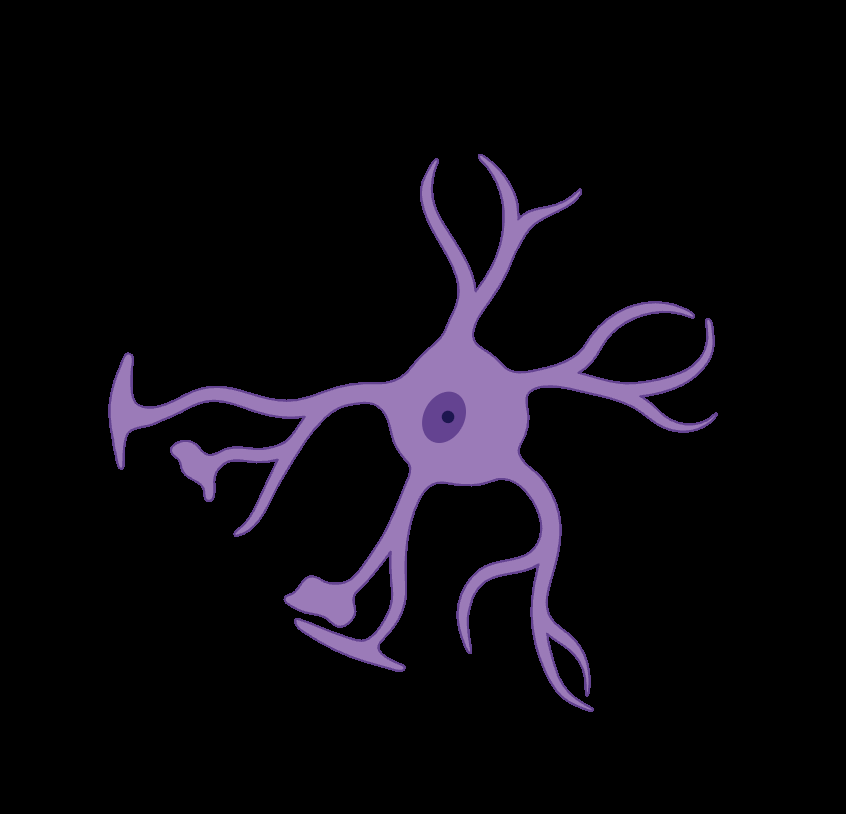
Fig 1: Schematic representation of glymphatic transport and clearance. Cerebrospinal fluid (CSF), produced by the choroid plexus via bulk

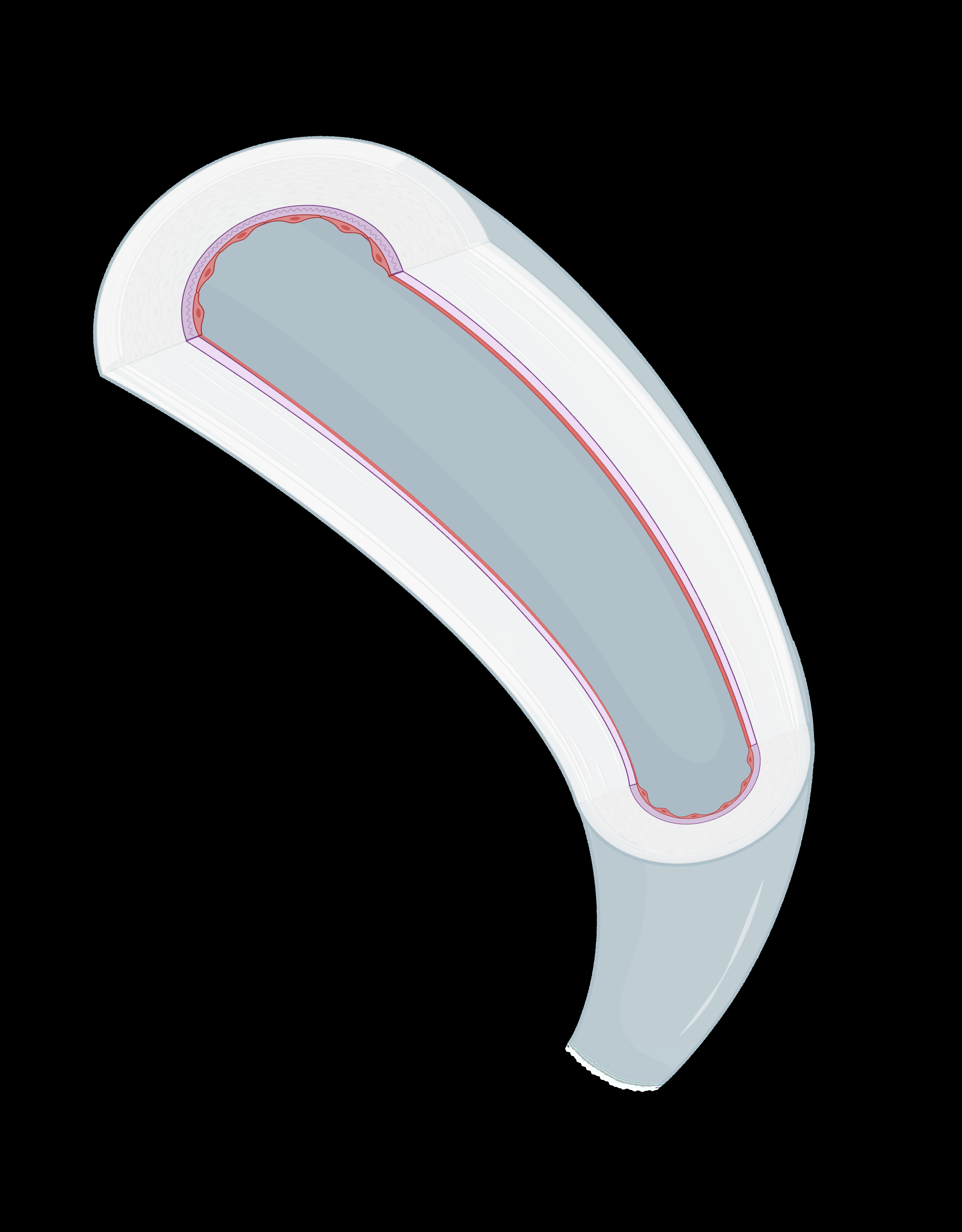
Fig 2 (page 4).

Fig 3 (page 4).

Fig 4 (page 4).

Fig 5 (page 4).

Fig 6 (page 4).

Fig 7 (page 4).

Fig 8 (page 4).

Limitations

• The excerpt provides no quantitative error table, so the strength of the improvement is mostly supported qualitatively by figures and agreement claims rather than reported RMSE/SSIM/etc.
• The evaluation appears to be on a single mouse CE-MRI experiment; generalization across animals, scanners, tracers, or disease states is not demonstrated in the provided text.
• The calibration window choice is heuristic: a five-step window is selected, but the authors explicitly say a formal sensitivity analysis is future work.
• The model assumes tracer clearance occurs through the boundary via a Robin condition, which may be an oversimplification of complex perivascular/lymphatic efflux pathways.
• The inverse problem depends on segmentation quality and immersed-domain discretization; segmentation errors or partial-volume effects could materially affect the recovered fields, but these are not deeply analyzed in the excerpt.
• It is unclear from the excerpt whether code, meshes, or inferred fields are released, which limits reproducibility and independent validation.

Open questions / follow-ons

• How sensitive are the recovered velocity, diffusivity, and clearance fields to the chosen calibration window and to tracer injection timing noise?
• Does the weakly divergence-free correction remain stable and identifiable under larger image noise, lower temporal sampling, or different tracers?
• Can the same inverse framework recover meaningful fields across multiple animals or pathological conditions, and how variable are the inferred clearance maps?
• How does this immersed IGA approach compare quantitatively with alternative regularized inverse methods, such as variational assimilation or Bayesian PDE inversion, on the same CE-MRI data?

Why it matters for bot defense

For a bot-defense engineer, the main transferable idea is not the glymphatic domain itself but the inverse-problem discipline: when reconstructing latent behavior from noisy observations, hard physical/structural constraints can matter more than raw fit. In CAPTCHA or abuse-detection systems, that maps to using constrained inference or consistency checks so estimated user/session behavior cannot violate invariants you already know must hold.

The paper is also a reminder that naive finite-difference-style estimation from sparse logs can be dominated by noise and discretization artifacts. If a defense pipeline reconstructs trajectories, typing dynamics, or interaction flows from event streams, enforcing conservation-like constraints, boundary conditions, or smoothness priors may yield more robust signals than unconstrained regression. The caution is that the method trades flexibility for physics: if the assumptions are wrong, the reconstruction can be beautifully consistent and still systematically biased, so validation on held-out temporal windows and across subjects is essential.

Cite

@article{arxiv2605_00730,
  title={ Reconstruction of glymphatic transport fields from subject-specific imaging data, with particular emphasis on cerebrospinal fluid flow and tracer conservation },
  author={ A. Derya Bakiler and Michael J. Johnson and Michael R. A. Abdelmalik and Frimpong A. Baidoo and Andrew Badachhape and Ananth V. Annapragada and Thomas J. R. Hughes and Shaolie S. Hossain },
  journal={arXiv preprint arXiv:2605.00730},
  year={ 2026 },
  url={https://arxiv.org/abs/2605.00730}
}

Read the full paper

• arXiv:2605.00730 (abstract)
• arXiv:2605.00730 (PDF)