An adaptive wavelet-based PINN for problems with localized high-magnitude source

Source: arXiv:2604.28180 · Published 2026-04-30 · By Himanshu Pandey, Ratikanta Behera

TL;DR

This paper targets a very specific failure mode of PINNs: when the PDE forcing is extremely localized and large in magnitude, the residual loss can dwarf boundary/initial losses by many orders of magnitude, so standard PINN training gets stuck fitting the easiest terms while missing the sharp source-driven features. The authors argue that existing fixes either require careful, problem-specific loss reweighting or become memory-heavy when using dense wavelet bases at high resolution.

Their proposal, AW-PINN, starts from a wavelet PINN pretraining phase and then makes the wavelet family itself adaptive: it selects physically relevant basis families using similarity between each family’s response and the PDE source/boundary terms, then fine-tunes scales and translations directly as learnable parameters. They also avoid autograd for derivatives by differentiating the wavelet basis analytically. Empirically, on four PDE families with loss ratios up to 10^10:1, AW-PINN consistently gives the lowest relative L2 error among the compared methods and is typically faster than the prior wavelet/balancing baselines, though not always the fastest wall-clock method.

Key findings

• On the transient heat equation with localized source, at ε=0.12 AW-PINN reaches relative L2 error 3.52 ± 0.81 × 10^-6, versus 4.05 ± 0.38 × 10^-5 for W-PINN and 1.71 ± 0.53 × 10^-5 for MMPINN (Table 4.1).
• On the same heat problem at ε=0.10, AW-PINN achieves 8.86 ± 0.87 × 10^-6; W-PINN is 3.10 ± 0.86 × 10^-5 and MMPINN is 8.46 ± 0.68 × 10^-1, with MMPINN reported as ineffective to converge (Table 4.1).
• For the 2D localized Poisson problem at ε=0.02, AW-PINN gets 2.68 ± 0.53 × 10^-4, compared with 9.81 ± 1.72 × 10^-3 for W-PINN and 3.25 ± 1.16 × 10^-3 for MMPINN (Table 4.2).
• For the Poisson problem at ε=0.05, AW-PINN gets 3.42 ± 0.13 × 10^-5 versus 3.55 ± 0.26 × 10^-4 for W-PINN and 5.71 ± 1.53 × 10^-4 for MMPINN (Table 4.2).
• For the oscillatory flow equation, AW-PINN reaches 5.17 ± 0.61 × 10^-4, while W-PINN is 1.27 ± 0.15 × 10^-2 and MMPINN is 8.35 ± 0.97 × 10^-2 (Table 4.3).
• The heat-equation setup reports an initial loss ratio of Lb:Li:Lr = 1:10:10^9 at ε=0.1, illustrating the extreme imbalance AW-PINN is designed to handle.
• AW-PINN uses only 1000 Adam iterations plus L-BFGS for the heat cases, while MMPINN needed up to 200000 collocation-related counts in Table 4.1 and still failed at ε=0.10; AW-PINN’s reported training time was 24.14–25.52 min versus up to 208.36 min for MMPINN on the same benchmark.
• The paper reports averaging over 5–10 independent runs and gives mean ± standard deviation, which suggests some attention to initialization sensitivity, though no formal significance test is reported.

Methodology — deep read

The target threat model here is not adversarial in the security sense; it is numerical optimization failure in PINNs under extreme multiscale forcing. The authors assume a PDE is known, along with boundary/initial conditions and a set of collocation points. The problem is that the residual source term can be orders of magnitude larger than boundary or initial losses, so a standard PINN, or even a loss-rebalanced PINN, may overfit the dominant term and miss localized structure. Their assumption is that the relevant localized behavior can be represented well by a sparse subset of wavelet families, and that those families can be identified from a short pretraining phase.

The data are synthetic PDE benchmark problems with analytic or closed-form reference solutions. There is no external dataset in the machine-learning sense. The paper evaluates four PDE families: a 1D transient heat equation with a sharply peaked time-dependent source (Eq. 25), a 2D Poisson equation with a localized Gaussian source/solution (Eq. 26), a 1D linear advection/flow equation with a strong oscillatory source (Eq. 27), and a TEz Maxwell system in a rectangular cavity with a point-charge-like Gaussian pulse source (the full source/equation details are truncated in the excerpt, but the paper states this benchmark explicitly). For each problem they sample residual points in the PDE interior and supervised points on the boundary/initial conditions. Table 4.1 uses NI/NB/NR to denote numbers of initial, boundary, and residual points; for example, the heat benchmark at ε=0.12 uses NI=1000, NB=2000, NR=20000 for AW-PINN, while the baseline PINN uses 5000/10000/50000. Table 4.2 and Table 4.3 similarly specify NB/NR and NI/NB/NR. Preprocessing is not elaborate: the main “data” are collocation locations and the corresponding PDE right-hand side values at those locations.

Architecturally, AW-PINN is a two-stage extension of the authors’ earlier W-PINN. Stage 1 is a fixed-basis W-PINN pretraining phase. The solution is represented as a sum over wavelet basis functions Ψ_i(x) with trainable coefficients c_i, plus a bias term B. The basis functions are separable tensor-product wavelets formed from a mother wavelet ψ and dyadic scale/translation parameters (Eq. 4–8). In the paper they use the Gaussian wavelet, defined as the first derivative of a Gaussian, citing its smoothness and localization. The model minimizes the usual PINN loss L = L_res + L_sup, but derivatives of the PDE residual are computed analytically from the wavelet basis rather than via automatic differentiation, which is a central design choice inherited from W-PINN. The novelty in AW-PINN is that after pretraining, the method scores each wavelet family by how well its residual response R_i and boundary response B_i align with the PDE right-hand side f and boundary data g, using similarity scores Score_i^R and Score_i^B (Eq. 15–16). Families with strong similarity and the top κ coefficients are kept as the active set I_A.

Stage 2 replaces each selected fixed family with an adaptive wavelet unit W_i(x; θ_i)=∏n ψ(w x_n + b_{i,n}) (Eq. 18), where the initial scale and translation are seeded from the selected dyadic parameters via w_{i,n}^{(0)}=2^{j_{i,n}} and b_{i,n}^{(0)}=-k_{i,n}. The final approximation is ˆu_Aψ(x;θ)=Σ_i c_i(θ) W_i(x;θ_i)+B (Eq. 19). This means the basis is no longer fixed; the scale/shift parameters themselves are optimized so the model can “move” resolution where the PDE needs it instead of populating a full high-resolution basis globally. The paper also derives an infinite-family Gaussian process limit for the adaptive model under random initialization and bias B=0 (Theorem 1), and decomposes the empirical NTK into a term from the linear coefficients c_i and a term from the adaptive parameters θ_i (Eq. 20–23). The theorem is mostly theoretical support; it does not appear to be used operationally in training.

Training is done with Adam during the pretraining stage and L-BFGS during the adaptive refinement stage. The excerpt gives one concrete example: for the heat-conduction benchmark they run 5000 Adam iterations for W-PINN pretraining, described as about two minutes, then switch to L-BFGS for AW-PINN until convergence. For W-PINN and MMPINN, they also use a few Adam epochs followed by L-BFGS. All parameters are initialized with Xavier initialization. The experiments are repeated five to ten times independently to reduce sensitivity to initialization, and the paper reports mean ± standard deviation. The implementation uses PyTorch 2.6.0 + CUDA 12.4 on an NVIDIA RTX A6000 GPU. Hyperparameter details are said to be in Appendix A, but the excerpt does not include the exact learning rates, batch sizes, or L-BFGS settings, so those specifics are not recoverable here.

Evaluation is straightforward and domain-appropriate: they report relative L2 error on uniformly sampled test points across the domain, comparing predicted ˆu against analytic/reference u. Baselines are the plain PINN, W-PINN, and MMPINN. There are no hidden attacker splits or cross-validation; instead the main comparison is on problem instances with different ε values or source strengths. The paper also shows qualitative plots: for the heat benchmark, Fig. 4.2 shows the source, prediction, and pointwise absolute error; Fig. 4.3 shows loss trajectories and relative L2 error curves, with shaded standard deviations across 10 runs. For the Poisson benchmark, Fig. 4.4 shows source, exact solution, and pointwise errors; Fig. 4.5 shows scale adaptation, comparing the fixed W-PINN dyadic scales to the adapted scales learned by AW-PINN. For the flow benchmark, Fig. 4.6 shows source, prediction, absolute error, and cross-section comparisons. One concrete end-to-end example is the ε=0.1 heat case: a localized source creates a sharp transient around t≈0.5, the initial loss imbalance is 1:10:10^9, W-PINN is pretrained for 5000 Adam steps, active wavelet families are selected from the pretraining coefficients and similarity scores, the adaptive units are initialized from those selected scales/translates, and then L-BFGS refines both coefficients and wavelet parameters using analytic derivatives. The result is a low pointwise error across the domain and the best relative L2 among the compared methods.

Reproducibility is partial. The paper states that source code will be made available on request, which is weaker than a public repository with frozen weights and scripts. It does not report public datasets because the benchmarks are synthetic. The excerpt includes enough structural detail to reimplement the method, but some critical training specifics are deferred to an appendix not included here, and the Maxwell benchmark description is truncated. The theoretical derivation of the GP/NTK limit is provided, but the practical training gains are empirical rather than derived from that theory.

Technical innovations

• A two-stage wavelet PINN that first pretrains on a fixed wavelet basis and then adapts only the physically relevant families instead of instantiating a dense multiresolution basis everywhere.
• A family-selection heuristic based on similarity between each basis family’s PDE/boundary response and the actual right-hand side, plus retention of the top-κ coefficient magnitudes.
• An adaptive wavelet unit with learnable scale and translation parameters initialized from dyadic wavelet indices, allowing local refinement without full-domain wavelet-matrix growth.
• Closed-form analytic differentiation of the wavelet activations so the PINN residual can be trained without automatic differentiation, inheriting the efficiency idea from W-PINN.
• A Gaussian-process-limit and NTK decomposition for the adaptive wavelet model under infinite-family scaling, giving a kernel-theoretic view of the training dynamics.

Datasets

• Synthetic transient heat conduction benchmark — 1D PDE with ε ∈ {0.12, 0.11, 0.10}; training sizes reported as NI/NB/NR = 1000/2000/20000 for AW-PINN (problem-specific tables).
• Synthetic localized Poisson benchmark — 2D PDE with ε ∈ {0.05, 0.02}; training sizes reported as NB/NR = 4000/10000 and 4000/15000 for W-PINN, with AW-PINN using 4000/10000.
• Synthetic oscillatory flow benchmark — 1D advection equation with A=100, Ts=0.05; training sizes reported as NI/NB/NR = 1000/1000/20000 for AW-PINN.
• Synthetic Maxwell TEz benchmark — 3D spacetime cavity problem with a localized Gaussian pulse source; specific sample counts are not visible in the excerpt.

Baselines vs proposed

• Baseline PINN: heat ε=0.12 relative L2-error = 8.1 ± 1.32 × 10^-1 vs proposed = 3.52 ± 0.81 × 10^-6
• W-PINN: heat ε=0.12 relative L2-error = 4.05 ± 0.38 × 10^-5 vs proposed = 3.52 ± 0.81 × 10^-6
• MMPINN: heat ε=0.12 relative L2-error = 1.71 ± 0.53 × 10^-5 vs proposed = 3.52 ± 0.81 × 10^-6
• W-PINN: Poisson ε=0.02 relative L2-error = 9.81 ± 1.72 × 10^-3 vs proposed = 2.68 ± 0.53 × 10^-4
• MMPINN: Poisson ε=0.02 relative L2-error = 3.25 ± 1.16 × 10^-3 vs proposed = 2.68 ± 0.53 × 10^-4
• W-PINN: flow benchmark relative L2-error = 1.27 ± 0.15 × 10^-2 vs proposed = 5.17 ± 0.61 × 10^-4
• MMPINN: flow benchmark relative L2-error = 8.35 ± 0.97 × 10^-2 vs proposed = 5.17 ± 0.61 × 10^-4

Figures from the paper

Figures are reproduced from the source paper for academic discussion. Original copyright: the paper authors. See arXiv:2604.28180.

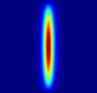
Fig 4: 2. Left to Right: Heat source function, the prediction using AW-PINN and respective absolute point-wise

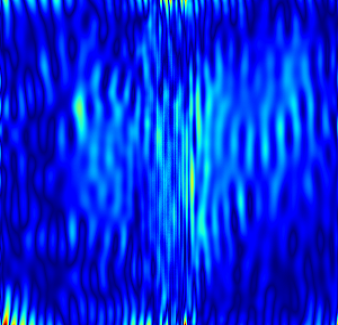
Fig 2 (page 10).

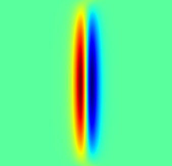
Fig 3 (page 10).

Fig 4 (page 12).

Fig 5 (page 12).

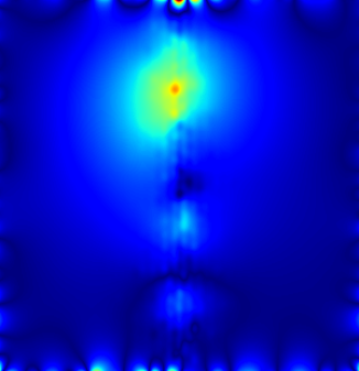
Fig 6 (page 12).

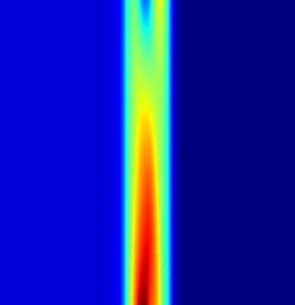
Fig 7 (page 12).

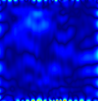
Fig 8 (page 12).

Limitations

• The source excerpt truncates the Maxwell benchmark details, so the exact PDE form, source specification, and quantitative result table cannot be fully verified here.
• The paper says code will be made available on request rather than via a public repository, which weakens reproducibility.
• Several training details are deferred to Appendix A and are not visible in the excerpt, including exact hyperparameters, so replication from the main text alone is incomplete.
• The method is validated on synthetic PDE benchmarks with analytic solutions, not on noisy measurements, inverse problems, or real-world data.
• The selection heuristic for active wavelet families is based on response similarity and top coefficient magnitudes, but the sensitivity of that heuristic to κ or to noisy residual estimates is not fully explored.
• The paper demonstrates stronger accuracy and often lower wall time than W-PINN/MMPINN, but does not report statistical significance tests beyond mean ± standard deviation.

Open questions / follow-ons

• How sensitive is the family-selection step to the threshold κ, especially when the PDE right-hand side is noisy, partially unknown, or only weakly localized?
• Can the adaptive wavelet idea be extended to inverse problems or data assimilation, where the source term itself is not fully specified?
• Does the analytic-derivative advantage persist for higher-dimensional PDEs with more complex geometries, where wavelet basis construction and derivative expressions may become cumbersome?
• How does AW-PINN compare to more modern PINN balancing methods or adaptive sampling schemes on the same localized-source benchmarks?

Why it matters for bot defense

For bot-defense and CAPTCHA work, this paper is not directly about adversaries or classification, but it is relevant as an optimization pattern: if a model must learn sparse, localized, high-magnitude signals, a fixed basis or uniform-resolution representation may waste capacity globally and still miss the rare hard regions. The adaptive-wavelet idea suggests a general strategy for localized anomaly detection or challenge-response modeling: start with a coarse representation, identify the few components that matter most, and then adapt resolution only where the signal demands it.

A CAPTCHA engineer should also note the methodological cautionary tale: when one loss term is orders of magnitude larger than others, naive training can look stable while failing on the rare cases that matter. The paper’s two-stage selection/refinement and its analytic-derivative setup are concrete reminders that sparse, high-frequency, or highly localized phenomena often benefit from architectural bias plus targeted adaptation rather than only from reweighting the objective.

Cite

@article{arxiv2604_28180,
  title={ An adaptive wavelet-based PINN for problems with localized high-magnitude source },
  author={ Himanshu Pandey and Ratikanta Behera },
  journal={arXiv preprint arXiv:2604.28180},
  year={ 2026 },
  url={https://arxiv.org/abs/2604.28180}
}

Read the full paper

• arXiv:2604.28180 (abstract)
• arXiv:2604.28180 (PDF)